We have discussed quite a few different orthogonal transforms, including
Fourier transform, cosine transform, Walsh-Hadamard transform, Haar transform,
etc., each of which, in its discrete form, is associated with an orthogonal
(or unitary) matrix ![]() that satisfies
that satisfies
![]() or
or
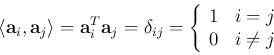
![]() . This orthogonal matrix can
be expressed in terms of its
. This orthogonal matrix can
be expressed in terms of its ![]() column vectors:
column vectors:
![\begin{displaymath}{\bf A}=[{\bf a}_1,\cdots,{\bf a}_{N}],\;\;\;\;\;\mbox{or}\;\...
... {\bf a}_1^T \vdots {\bf a}^T_{N}
\end{array} \right]
\end{displaymath}](img5.png)
We have seen several times in the previous discussions of the various
orthogonal transforms, the transform of any given discrete signal, represented
as a vector in the N-dimensional space spanned by the standard basis vectors
![\begin{displaymath}
{\bf x}=\left[\begin{array}{c}x_1 \vdots x_N\end{array}\...
...+x_N\left[\begin{array}{c}0 \vdots 0 1\end{array}\right]
\end{displaymath}](img7.png)
![\begin{displaymath}{\bf y}=\left[ \begin{array}{c}y_1 \vdots y_{N} \end{ar...
...}_1^T \vdots \\
{\bf a}^T_{N} \end{array} \right] {\bf x} \end{displaymath}](img8.png)
![\begin{displaymath}{\bf x}={\bf A}{\bf y}=[{\bf a}_1,\cdots,{\bf a}_{N}]
\left[ ...
...ots y_{N} \end{array} \right]
=\sum_{i=1}^{N} y_i {\bf a}_i \end{displaymath}](img13.png)
In the previous chapters, we have also seen some specific applications of each of the transforms, such as various filtering in the transform domain (e.g., in frequency domain by Fourier transform and discrete cosine transform), such as encoding and data compression. Do all of these transforms, each represented by a totally different transform matrix from others, share some intrinsic properties and essential characteristics in common? Moreover, we may want to ask some more general questions, why do we want to carry out such transforms to start with? If an orthogonal transform is nothing more than a certain rotation of the signal vector in the N-dimensional space, what can be achieved by such a rotation? And, finally, is there a best rotation among all possible transform rotations (infinitely many of them)?
The following discussion for the principal component analysis (PCA) and the associated Karhunen-Loeve Transform (KLT) will answer all these questions.