Covariance and Correlation

Let $x_i$ and $x_j$ be two real random variables in a random vector ${\bf x}=[x_1,\cdots,x_N]^T$. The mean and variance of a variable $x_i$ and the covariance and correlation coefficient (normalized correlation) between two variables $x_i$ and $x_j$ are defined below:

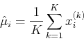
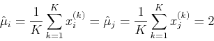
• Mean of $x_i$: $\mu_i=E(x_i)$
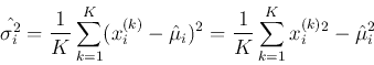
• Variance of $x_i$: $\sigma^2_i=E[ (x_i-\mu_i)^2 ]=E(x_i^2)-m_i^2$
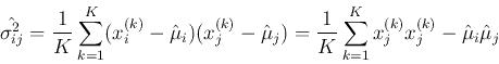
• Covariance of $x_i$ and $x_j$: $\sigma^2_{ij}=E[ (x_i-\mu_i)(x_j-\mu_j) ]=E(x_ix_j)-\mu_i\mu_j$
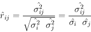
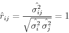
• Correlation coefficient between $x_i$ and $x_j$: $r_{ij}=\sigma_{ij}^2 / \sqrt{ \sigma_i^2\;\sigma_j^2} =\sigma_{ij}^2 / \sigma_i\;\sigma_j$

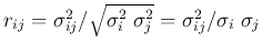
Note that the correlation coefficient $r_{ij}=\sigma^2_{i}/\sigma_i\sigma_j$ can be considered as the normalized covariance $\sigma^2_{ij}$.

To obtain these parameters as expectations of the first and second order functions of the random variables, the joint probability density function $p(x_1,\cdots,x_N)$ is required. However, when it is not available, the parameters can still be estimated by averaging the outcomes of a random experiment involving these variables repeated $K$ times:

$$\hat{\mu}_i=\frac{1}{K}\sum_{k=1}^K x_i^{(k)}$$

$$\hat{\sigma^2_i}=\frac{1}{K}\sum_{k=1}^K (x_i^{(k)}-\hat{\mu}_i)^2 =\frac{1}{K}\sum_{k=1}^K x_i^{(k)}^2-\hat{\mu}_i^2$$

$$\hat{\sigma^2_{ij}}=\frac{1}{K}\sum_{k=1}^K (x_i^{(k)}-\hat{... ...c{1}{K}\sum_{k=1}^K x_j^{(k)}x_j^{(k)}-\hat{\mu}_i \hat{\mu}_j$$

$$\hat{r}_{ij}=\frac{\hat{\sigma^2_{ij}}}{\sqrt{ \hat{\sigma_i... ...=\frac{\hat{\sigma^2_{ij}}}{\hat{\sigma_i}\; \hat{\sigma_j} }$$

To understand intuitively the meaning of these parameters, we consider the following very simple examples.

Examples:

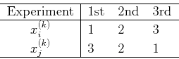
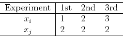
• Assume the experiment concerning $x_i$ and $x_j$ is repeated $K=3$ times with the following outcomes:
  
  $$\begin{tabular}{c\vert lll}\hline Experiment & 1st & 2nd & 3... ... 1 & 2 & 3 \\ $x_j^{(k)}$ & 1 & 2 & 3 \hline \end{tabular}$$
  
  
  The means, variances and covariance of $x_i$ and $x_j$ can be estimated as
  
  $$\hat{\mu}_i=\frac{1}{K}\sum_{k=1}^Kx_i^{(k)} =\hat{\mu}_j=\frac{1}{K}\sum_{k=1}^Kx_j^{(k)}=2$$
  
  
  
  
  $$\hat{\sigma^2_i}=\frac{1}{K}\sum_{k=1}^K(x_i^{(k)}-\hat{\mu... ...1+2 \times 2+3 \times 3)/3-2 \times 2=0.667=\hat{\sigma^2_j}$$
  
  
  
  
  $$\hat{\sigma^2_{ij}}=\frac{1}{K}\sum_{k=1}^K(x_i^{(k)}-\hat{... ...u}_j =(1 \times 1+2 \times 2+3 \times 3)/3-2 \times 2=0.667$$
  
  
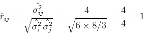
  and the correlation coefficient is:
  
  $$\hat{r}_{ij}=\frac{\hat{\sigma^2_{ij}}}{\sqrt{\hat{\sigma^2_i} \hat{\sigma^2_j}}}=1$$
  
  
  We see that $x_i$ and $x_j$ are highly (maximally in this case) correlated.

• Assume the outcomes of the 3 experiments are
  
  $$\begin{tabular}{c\vert lll}\hline Experiment & 1st & 2nd & 3... ... 2 & 4 & 6 \\ $x_j^{(k)}$ & 3 & 6 & 9 \hline \end{tabular}$$
  
  
  then we have
  
  $$\hat{\mu}_i=4,\;\;\hat{\mu}_j=6,\;\;\hat{\sigma^2_i}=8/3,\;\;\hat{\sigma^2_j}=6, \;\;\hat{\sigma^2_{ij}}=4$$
  
  
  and
  
  $$\hat{r}_{ij}=\frac{\hat{\sigma^2_{ij}}}{\sqrt{\hat{\sigma^2_i} \hat{\sigma^2_j}}} =\frac{4}{\sqrt{6\times 8/3}}=\frac{4}{4}=1$$
  
  
  We see that the two variables $x_i$ and $x_j$ can be individually scaled while their correlation remains the same.
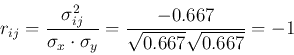
• Assume the outcomes of the 3 experiments are
  
  $$\begin{tabular}{c\vert lll}\hline Experiment& 1st & 2nd & 3rd... ... 1 & 2 & 3 \\ $x_j^{(k)}$ & 3 & 2 & 1 \hline \end{tabular}$$
  
  
  We have $\hat{\mu}_i=\hat{\mu}_j=2$ and
  
  $$\hat{\sigma^2_{ij}}=\frac{1}{K}\sum_{k=1}^K(x_i^{(k)}-\hat{\... ...mu}_j =(1 \times 3+2 \times 2+3 \times 1)/3-2 \times 2=-0.667$$
  
  
  
  
  $$\hat{\sigma}^2_x=\hat{\sigma}^2_y=0.667$$
  
  
  And the correlation coefficient is:
  
  $$r_{ij}=\frac{\sigma_{ij}^2}{\sigma_x \cdot \sigma_y} =\frac{-0.667}{\sqrt{0.667}\sqrt{0.667}}=-1$$
  
  
  indicating that the two variables are highly inversely correlated.

• Assume the outcomes are:
  
  $$\begin{tabular}{c\vert lll}\hline Experiment& 1st & 2nd & 3rd... ...x_i$ & 1 & 2 & 3 \\ $x_j$ & 2 & 2 & 2 \hline \end{tabular}$$
  
  
  We have $\hat{\mu}_i=\hat{\mu}_j=2$, $\hat{\sigma_i}=\hat{\sigma_i}=\hat{\sigma_{ij}}=0.667$ and
  
  $$\hat{\sigma^2_{ij}}=(1 \times 2+2 \times 2+3 \times 2)/3-2 \times 2=0$$
  
  
  and $r_{ij}=0$, indicating that the two variables are totally uncorrelated (unrelated).

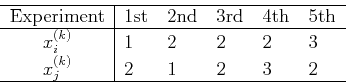
• Assume the experiment is carried out $K=5$ times with the outcomes:
  
  $$\begin{tabular}{c\vert lllll}\hline Experiment& 1st & 2nd & 3... ... 3 \\ $x_j^{(k)}$ & 2 & 1 & 2 & 3 & 2 \hline \end{tabular}$$
  
  
  We still have
  
  $$\hat{\mu}_i=\hat{\mu}_j=2$$
  
  
  
  
  $$\hat{\sigma^2_{ij}}=(1 \times 2+2 \times 1+2 \times 2+2 \times 3+3 \times 2)/5 -2 \times 2=0$$
  
  
  and $r_{ij}=0$, indicating that the two variables are totally uncorrelated (unrelated).

Now we see that the covariance $\sigma_{ij}^2$ represents how much the two ramdom variables $x_i$ and $x_j$ are positively correlated if $\sigma_{ij}^2>0$, negatively correlated if $\sigma_{ij}^2<0$, or not correlated at all if $\sigma_{ij}^2=0$.

Assume a random vector ${\bf x}=[x_1,\cdots,x_N]^T$ is composed of $N$ samples of a signal $x(t)$. The signal samples close to each other tend to be more correlated than those that are farther away, i.e., given $x_i$, we can predict the next sample $x_{i+1}$ with much higher confidence than predicting some $x_j$ which is farther away. Consequently, the elements in the covariance matrix ${\bf\Sigma}_x$ near the main diagonal have higher values than those farther away from the diagonal.