Karhunen-Loeve Transform (KLT)

Now we consider the Karhunen-Loeve Transform (KLT) (also known as Hotelling Transform and Eigenvector Transform), which is closely related to the Principal Component Analysis (PCA) and widely used in data analysis in many fields.

Let ${\bf\phi}_k$ be the eigenvector corresponding to the kth eigenvalue $\lambda_k$ of the covariance matrix ${\bf\Sigma}_x$, i.e.,

$${\bf\Sigma}_x {\bf\phi}_k=\lambda_k{\bf\phi}_k\;\;\;\;\;\;(k=1,\cdots,N)$$

or in matrix form:

$$\left[ \begin{array}{ccc}\cdots &\cdots &\cdots \\ \cdots & ... ...f\phi}_k \end{array} \right] \;\;\;\;\;\;(k=1,\cdots,N)$$

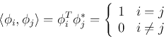
As the covariance matrix ${\bf\Sigma}_x={\bf\Sigma}_x^{*T}$ is Hermitian (symmetric if ${\bf x}$ is real), its eigenvector ${\bf\phi}_i$'s are orthogonal:

$$\langle {\bf\phi}_i,{\bf\phi}_j\rangle={\bf\phi}^T_i {\bf\phi... ...\{ \begin{array}{ll} 1 & i=j 0 & i\ne j \end{array} \right.$$

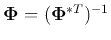
and we can construct an $N \times N$ unitary (orthogonal if ${\bf x}$ is real) matrix ${\bf\Phi}$

$${\bf\Phi}\stackrel{\triangle}{=}[{\bf\phi}_1, \cdots,{\bf\phi}_{N}]$$

satisfying

$${\bf\Phi}^{*T} {\bf\Phi} = {\bf I},\;\;\;\;\mbox{i.e.,}\;\;\;\; {\bf\Phi}^{-1}={\bf\Phi}^{*T}$$

The $N$ eigenequations above can be combined to be expressed as:

$${\bf\Sigma}_x{\bf\Phi}={\bf\Phi}{\bf\Lambda}$$

or in matrix form:

$$\left[ \begin{array}{ccc}\ddots &\cdots &\cdots \\ \vdots &... ... & \vdots \\ 0 & \cdots & \lambda_{N} \end{array} \right]$$

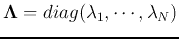
Here ${\bf\Lambda}$ is a diagonal matrix ${\bf\Lambda}=diag(\lambda_1, \cdots, \lambda_{N} )$. Left multiplying ${\bf\Phi}^T={\bf\Phi}^{-1}$ on both sides, the covariance matrix ${\bf\Sigma}_x$ can be diagonalized:

$${\bf\Phi}^{*T}{\bf\Sigma}_x{\bf\Phi}={\bf\Phi}^{-1} {\bf\Sigm... ... {\bf\Phi} = {\bf\Phi}^{-1}{\bf\Phi}{\bf\Lambda}={\bf\Lambda}$$

Now, given a signal vector ${\bf x}$, we can define a unitary (orthogonal if ${\bf x}$ is real) Karhunen-Loeve Transform of ${\bf x}$ as:

$${\bf y}=\left[ \begin{array}{c} y_1 \vdots y_{N} \end{... ...ht]\left[\begin{array}{c}x_1 \vdots, x_N\end{array}\right]$$

where the ith component $y_i$ of the transform vector is the projection of ${\bf x}$ onto ${\bf\phi_i}$:

$$y_i=\langle {\bf\phi}_i,{\bf x} \rangle={\bf\phi}_i^T{\bf x}^*$$

Left multiplying ${\bf\Phi}=({\bf\Phi}^{*T})^{-1}$ on both sides of the transform ${\bf y}={\bf\Phi}^{*T} {\bf x}$, we get the inverse transform:

$${\bf x}={\bf\Phi} {\bf y}=\left[\begin{array}{ccc}&& {\bf... ...dots y_{N} \end{array} \right] =\sum_{i=1}^{N} y_i \phi_i$$

We see that by this transform, the signal vector ${\bf x}$ is now expressed in an N-dimensional space spanned by the N eigenvectors ${\bf\phi}_i$ ($i=1,\cdots,N$) as the basis vectors of the space.