Geometric Interpretation of KLT

Assume the N random variables in a signal vector ${\bf x}=[x_1,\cdots, x_{N}]^T$ have a normal joint probability density function:

$$p(x_1,\cdots, x_{N})=p({\bf x})=N({\bf x}, {\bf m}_x, {\bf\S... ...bf x}-{\bf m}_x)^T{\bf\Sigma}_x^{-1}({\bf x}-{\bf m}_x)\right]$$

where ${\bf m}_x$ and ${\bf\Sigma}_x$ are the mean vector and covariance matrix of ${\bf x}$, respectively. When $N=1$, ${\bf\Sigma}_x$ and ${\bf m}_x$ become ${\bf\sigma}^2_x$ and $\mu_x$, respectively, and the density function becomes the familiar single variable normal distribution:

$$p(x)=N(x,\mu_x, \sigma_x) =\frac{1}{\sqrt{2\pi \sigma_x^2}}\;exp\left[-\frac{(x-\mu_x)^2}{2\sigma_x^2}\right]$$

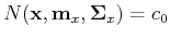
The shape of this normal distribution in the N-dimensional space can be represented by the iso-hypersurface in the space determined by equation

$$N({\bf x},{\bf m}_x,{\bf\Sigma}_x)=c_0$$

where $c_0$ is a constant. Or, equivalently, this equation can be written as

$$({\bf x}-{\bf m}_x)^T {\bf\Sigma}_x^{-1} ({\bf x}-{\bf m}_x) = c_1$$

where $c_1$ is another constant related to $c_0$, ${\bf m}_x$ and ${\bf\Sigma}_x$.

In particular, when $N=2$, ${\bf x}=[x_1, x_2]^T$, and we assume

$${\bf\Sigma}_x^{-1}=\left[ \begin{array}{cc} A & B/2 B/2 & C \end{array} \right]$$

then the equation above becomes

$$({\bf x}-{\bf m}_x)^T {\bf\Sigma}_x^{-1} ({\bf x}-{\bf m}_x) = [x_1-\mu_{x_1}, x_2-\mu_{x_2}] \left[ \begin{array}{cc} A & B/2 ... ...] \left[ \begin{array}{c} x_1-\mu_{x_1} x_2-\mu_{x_2} \end{array} \right]$$

$$= A(x_1-\mu_{x_1})^2+B(x_1-\mu_{x_1})(x_2-\mu_{x_2})+C(x_2-\mu_{x_2})^2 = c_1$$

As ${\bf\Sigma}_x$ is positive definite, and so is ${\bf\Sigma}_x^{-1}$, we have

$$\left\vert {\bf\Sigma}_x^{-1} \right\vert = AC-B^2/4 > 0$$

i.e., the quadratic equation above represents an ellipse (instead of other quadratic curves such as hyperbola and parabola) centered at ${\bf m}_x=[\mu_1, \mu_2]^T$. When $N=3$, the quadratic equation represents an ellipsoid. In general when $N>3$, the equation $N({\bf x}, {\bf m}_x, {\bf\Sigma}_x)=c_0$ represents a hyper ellipsoid in the N-dimensional space. The center and spatial distribution of this ellipsoid are determined by ${\bf m}_x$ and ${\bf\Sigma}_x$, respectively.

By the KLT, the signal ${\bf y}={\bf\Phi}^T {\bf x}$ is completely decorrelated and its the covariance matrix becomes diagonalized:

$${\bf\Sigma}_y ={\bf\Lambda}= \left[ \begin{array}{ccc} \la... ... \vdots \\ 0 & \cdots & \sigma^2_{y_{N}} \end{array} \right]$$

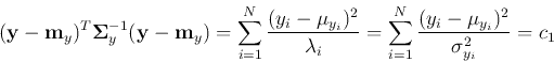
and the isosurface equation 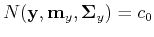$N({\bf y},{\bf m}_y, {\bf\Sigma}_y)=c_0$ becomes

$$({\bf y}-{\bf m}_y)^T{\bf\Sigma}_y^{-1}({\bf y}-{\bf m}_y) ... ...\sum_{i=1}^{N} \frac{(y_i-\mu_{y_i})^2}{\sigma^2_{y_i}} =c_1$$

This equation represents a standard hyper-ellipsoid in the N-dimensional space. In other words, the KLT ${\bf y}={\bf\Phi}^T {\bf x}$ rotates the coordinate system so that the semi-principal axes of the ellipsoid represented by $N({\bf x},{\bf m}_x,{\bf\Sigma}_x)=C$ are in parallel with ${\bf\phi}_i$ ( $i=1,\cdots,N$), the axes of the new coordinate system. Moreover, the length of the semi-principal axis parallel to ${\bf\phi}_i$ is proportional to $\sqrt{\lambda_i}=\sigma_{y_i}$.

The standardization of the ellipsoid is the essential reason why the rotation of KLT can achieve two highly desirable outcomes: (a) the decorrelation of the signal components, and (b) redistribution and compaction of the energy or information contained in the signal, as illustrated in the figure: