Applications

Here are some examples of the applications of KLT in image processing and recognition.

• Remote sensing data compression

  In remote sensing, pictures of the surface of either the Earth or other planets such as Mars are taken by satellites, for various studies (e.g., geology, geography, etc.). The camera system on the satellite has an array of $N$ sensors, typically a few tens or even over a hundred, each of which is sensitive to a different wavelength band in the visible and infrared range of the electromagnetic spectrum. These sensors will produce a set of $N$ images all covering the same surface area on the ground. For the same pixel in these images, there are $N$ values (each from one wavelength band) representing the spectral profile that characterizes the material on the surface area corresponding to the pixel. Depending on the number of sensors $N$, the data are referred to as either multi or hyper-spectral images.

  As different types of materials on the ground surface usually have different spectral profiles, one typical application of the multi or hyper-spectral image data is to classify the pixels into different materials. When $N$ is large, KLT can be used to reduce the dimensionality without loss of much useful information. Specifically, we consider the $N$ values associated with each pixel form an N-dimensional random vector, and then carry out KLT to reduce its dimensionality to $M«N$. All classification will subsequently carried out in this low dimensional space, thereby significantly reducing the computational complexity.

  

  

• Vedio image compression

  A sequence of $N=8$ frames of a video of a moving escalator and their eigen-images are shown respectively in the upper and lower parts of the figure below

  

  The covariance matrix and the energy distribution among the eight components plot both before and after the KLT are shown in this figure

  

  We see that due to the local correlation, the covariance matrix before the KLT (left) does indeed resemble the correlation matrix R of a first-order Markov model (bottom right in Fig. 9.12), and the covariance matrix after the KLT (middle) is completely decorrelated and its energy highly compacted, as also clearly shown in the comparison of the energy distribution before and after the KLT (right). Also as shown in Eq. (9.18), the KLT basis, the set of all N = 8 eigenvectors of the signal covariance matrix, is very much similar to the DCT basis, indicating that the DCT with a fast algorithm would produce almost the same results as the KLT. Moreover, it is interesting to observe that the first eigen-image (left panel of the third row of Fig. 9.16 represents mostly the static scene of the image frames corresponding to the main variations in the image (carrying most of the energy), while the subsequent eigen-images represent mostly the motion in the video, the variation between the frames. For example, the motion of the people riding on the escalator is mostly reflected by the first few eigen-images following the first one, while the motion of the escalator stairs is mostly reflected in the subsequent eigen-images.

• Eigenfaces and face recognition

  Twenty images of faces ($N=20$):

  

  The eigen-images after KLT:

  

  Percentage of energy contained in the

  components	1	2	3	4	5	6	7	8	9	10	11	12	13	14	15	16	17	18	19	20
  percentage energy	48.5	11.6	6.1	4.6	3.8	3.7	2.6	2.5	1.9	1.9	1.8	1.6	1.5	1.4	1.3	1.2	1.1	1.1	0.9	0.8
  accumulative energy	48.5	60.1	66.2	70.8	74.6	78.3	81.0	83.5	85.4	87.3	89.	90.7	92.2	93.6	94.9	96.1	97.2	98.2	99.2	100.0

  Reconstructed faces using 95% of the total information (15 out of 20 components):

  

  The KLT can also be used for face recognition, where a face image of $K$ pixels is to be classified to be the same as one of the training images with known identities.

• Visualization and Feature extraction for pattern recognition

  In many applications, various objects, called patterns in the field of machine learning, in the images (e.g., hand-written characters, human faces, etc.) need to be classified. As the first step of this process, a set of features pertaining to the patterns of interest need to be extracted. KLT can be used for this purpose. Assume a set of images are taken, each containing one of the ten numbers from 0 to 9 (or the face of one individual). Each image is treated as a vector by concatenating all of its rows one after another. Next the mean vector and covariance matrix of these vectors are obtained. Based on the covariance matrix, the KLT is carried out to reduce the dimensionality of the vectors from $N$ to $«N$. Alternatively, to better extract the information pertaining to the difference between different classes of patterns, the KLT can be based on a different matrix called between-class scatter matrix, which represents the separability of the classes. Specifically, we use the eigenvectors corresponding to the $M$ largest eigenvalues of the between-class scatter matrix to form an $M$ by $N$ transform matrix. After the transform by this matrix, some classification algorithm can be carried out in the much reduced M-dimensional space.

  Example: The image below shows the ten numbers from 0 to 9 hand written by different students. Each number is represented by an image of $16\times 16=256$ pixels, which can be considered as an $N=256$ dimensional vector.

  

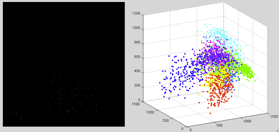
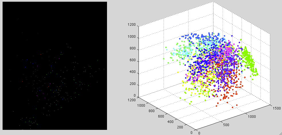
  To visualize the data set, the KLT based on the covariance matrix ${\bf\Sigma}_{N\times N}$ of the dataset is used to project the $N=256$ dimensional onto an $M\ll N$ dimensional space, as shown in the figure below with $M=2$ on the left and $M=3$ on the right. The sample vectors in each of the ten different classes are color-coded. It can be seen that even when the dimensions are much reducrf from $N=256$ to $M=3$, it is still possible to separate the ten different classes reasonably well.

  

  The following is obtained by the KLT based on the between-class scatter matrix ${\bf S}_B$, i.e., the classes should be more separable.