Next: Applications Up: klt Previous: Comparison with Other Orthogonal

KLT of images

Each of a set of images of rows and columns and $K=r\times c$ pixels can be represented as a K-D vector by concatenating its columns (or its rows), and the images can be represented by a $K\times N$ array ${\bf X}$ with each column for one of the images:

$\begin{displaymath} {\bf X}_{K\times N} =[{\bf x}_{c_1},\cdots,{\bf x}_{c_N}] ... ... ({\bf X}^T)_{N\times K}=[{\bf x}_{r_1},\cdots,{\bf x}_{r_K}] \end{displaymath}$

where ${\bf x}_c_i$ is a K-D column vector containing the

pixels of the ith image, and ${\bf x}_r_j^T$ is an N-D row vector containing the pixels at the same position of all

images. If ${\bf X}$ is not degenerate, its rank is

$\begin{displaymath} R=\Rank({\bf X})=\min(N,K) \end{displaymath}$

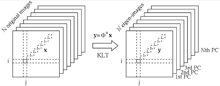
A KLT can be applied to either the column or row vectors of the data array ${\bf X}$ , depending on whether the column or row vectors are treated as the realizations (samples) of a random vector.

If the rows ${\bf x}_{r_i}$ ( $i=1,\cdots,K$ ) of ${\bf X}$ are treated as realizations of an N-D random vector ${\bf x}_r$ (assumed to have zero mean without loss of generality), its covariance matrix can be estimated by:

$\begin{displaymath} {\bf\Sigma}_r=\frac{1}{K}\sum_{i=1}^K{\bf x}_{r_i}{\bf x}^T... ...x}_{r_K}^T\end{array}\right] =\frac{1}{K} ({\bf X}^T{\bf X}) \end{displaymath}$

This is an $N \times N$ symmetric and positive semi-definite matrix of rank $R=\min(K,N)$ . Its eigenequation is:

$\begin{displaymath} ({\bf X}^T{\bf X}){\bf u}_i=\lambda_i{\bf u}_i,\;\;\;\;\;(i=1,\cdots,N) \end{displaymath}$

where $\lambda_i$ is the ith non-negative eigenvalue and ${\bf u}_i$ the corresponding N-D eigenvector. Note that the scaling factor is dropped. The eigenequation above can be expressed in matrix form as:

$\begin{displaymath} ({\bf X}^T{\bf X}){\bf U}={\bf U}{\bf\Lambda} \end{displaymath}$

where ${\bf\Lambda}=diag(\lambda_1,\cdots,\lambda_N)$ is the diagonal eigenvalue matrix containing real non-negative eigenvalues: $\lambda_1\ge\lambda_2\ge\cdots\ge\lambda_N\ge 0$ , and ${\bf U}=[{\bf u}_1,\cdots,{\bf u}_N]$ is the orthogonal eigenvector matrix satisfying ${\bf U}^T={\bf U}^{-1}$ . The KLT transform can be carried out to each of the row vectors of ${\bf X}$ :

$\begin{displaymath} {\bf y}_{r_i}={\bf U}^T{\bf x}_{r_i},\;\;\;\;\;(i=1,\cdots,K) \end{displaymath}$

or in matrix form:

$\begin{displaymath} \left[{\bf y}_{r_1},\cdots,{\bf y}_{r_K}\right] ={\bf U}^T... ...^T{\bf X}^T,\;\;\;\;\mbox{or}\;\;\;\; {\bf Y}={\bf X}{\bf U} \end{displaymath}$

Each resulting N-D vector ${\bf y}_{r_i}$ contains the pixels at the same position of the eigen-images, as shown below:

Pre-multiplying ${\bf X}$ on both sides of the eigenequation above we get

$\begin{displaymath} ({\bf XX}^T) {\bf X}{\bf U}= {\bf X}{\bf U}{\bf\Lambda} \;... ...mbox{or}\;\;\;\;\;\; ({\bf XX}^T){\bf V}={\bf V}{\bf\Lambda} \end{displaymath}$

which happens to be the eigenequation of ${\bf\Sigma}_c={\bf XX}^T$ with the same eigenvalues $\lambda_i$ , and the corresponding eigenvector matrix ${\bf V}={\bf X}{\bf U}$ . Comparing this with the KLT aobve ${\bf Y}={\bf X}{\bf U}$ , we see that ${\bf V}={\bf Y}$ , i.e., each eigenvector ${\bf v}_i$ of ${\bf\Sigma}_c={\bf XX}^T$ is actually an eigen-images obtained by the KLT.
Alternatively, if the columns ${\bf x}_{c_j}$ ( $j=1,\cdots,N$ ) of ${\bf X}$ are treated as realizations of a K-D random vector ${\bf x}_c$ (again assumed to have zero mean), its covariance matrix can be estimated by:

$\begin{displaymath} {\bf\Sigma}_c=\frac{1}{N} \sum_{i=1}^N{\bf x}_{c_i}{\bf x}^... ...f x}_{c_K}\end{array}\right] =\frac{1}{N} ({\bf X}{\bf X}^T) \end{displaymath}$

This is a $K\times K$ symmetric and positive semi-definite matrix of rank $R=\min(K,N)$ . Its eigenequation is:

$\begin{displaymath} {\bf XX}^T{\bf v}_i=\lambda_i{\bf v}_i,\;\;\;\;\;(i=1,\cdots,K) \end{displaymath}$

Note that the scaling factor is dropped. The eigenequation can be expressed in matrix form as:

$\begin{displaymath} {\bf XX}^T{\bf V}={\bf V}{\bf\Lambda} \end{displaymath}$

where ${\bf V}=[{\bf v}_1,\cdots,{\bf v}_K]$ is a $K\times K$ orthogonal eigenvector matrix satisfying ${\bf V}^T={\bf V}^{-1}$ . The KLT transform can be carried out to the column vectors of ${\bf X}$ :

$\begin{displaymath} {\bf z}_{c_j}={\bf V}^T{\bf x}_{c_j},\;\;\;\;\;(j=1,\cdots,N) \end{displaymath}$

or in matrix form:

$\begin{displaymath} \left[{\bf z}_{c_1},\cdots,{\bf z}_{c_N}\right] ={\bf V}^T... ...\;\;\;\;\;\;\mbox{i.e.}\;\;\;\;\;\; {\bf Z}={\bf V}^T{\bf X} \end{displaymath}$

Each of the resulting K-D vector ${\bf y}_{c_i}$ contains the pixels of one of the KLT of
Pre-multiplying ${\bf X}^T$ on both sides we get

$\begin{displaymath} ({\bf X}^T{\bf X}){\bf X}^T{\bf V}={\bf X}^T{\bf V}{\bf\Lam... ...r}\;\;\;\;\;\; ({\bf X}^T{\bf X}){\bf U}={\bf U}{\bf\Lambda} \end{displaymath}$

This is the eigenequation of ${\bf\Sigma}_r={\bf X}^T{\bf X}$ with the same eigenvalues $\lambda_i$ , and the corresponding $K\times K$ eigenvector ${\bf U}={\bf X}^T{\bf V}$ .

From these two cases we see that the eigenvalue problems associated with these two different covariance matrices ${\bf\Sigma}_r={\bf X}^T{\bf X}$ and ${\bf\Sigma}_c={\bf XX}^T$ are equivalent, in the sense that they have the same non-zero eigenvalues, and their eigenvectors are related by ${\bf V}={\bf X}{\bf U}$ or ${\bf U}={\bf X}^T{\bf V}$ . We can therefore solve the eigenvalue problem of either of the two covariance matrices, depending on which has lower dimension.

Owing to the nature of the KLT, most of the energy/information contained in the images, representing the variations among all images, is concentrated in the first few eigen-images corresponding to the greatest eigenvalues, while the remaining eigen-images can be omitted without losing much energy/information. This is the foundation for various KLT-based image compression and feature extraction algorithms. The subsequent operations such as image recognition and classification can be carried out in a much lower dimensional space after the KLT.

In image recognition, the goal is typically to classify or recognize objects of interest, such as hand-written alphanumeric characters, or human faces, represented in an image of pixels. As not all pixels are necessary for representing the image object, the KLT can be carried out to compact most of the information into a small number of components:

$\begin{displaymath} {\bf Z}={\bf V}^T{\bf X} \end{displaymath}$

where the transform matrix ${\bf V}$ is the eigenvector matrix of the covariance matrix ${\bf\Sigma}_c={\bf XX}^T$ :

$\begin{displaymath} {\bf XX}^T{\bf V}={\bf V}{\bf\Lambda} \end{displaymath}$

When $K\ll N$ , the KLT matrix ${\bf V}$ can be obtained by directly solving this eigenvalue problem of the $K\times K$ covariance matrix. However, when $K\gg N$ , the complexity of this eigenvalue problem may be too high. In this case we can obtain the KLT matrix by ${\bf V}={\bf XU}$ as shown above, where ${\bf U}$ is the $N \times N$ eigenvector matrix of ${\bf\Sigma}_r={\bf X}^T{\bf X}$ :

$\begin{displaymath} {\bf X}^T{\bf XU}={\bf U}{\bf\Lambda} \end{displaymath}$

This eigenvalue problem can be more easily solved if $N\ll K$ . Now the desired KLT can be carried out as

$\begin{displaymath} {\bf z}={\bf V}^T{\bf X}=({\bf XU})^T{\bf X}={\bf U}^T({\bf... ... X}){\bf U}]^T=({\bf U}{\bf\Lambda})^T ={\bf\Lambda}{\bf U}^T \end{displaymath}$

Example

$\begin{displaymath} {\bf X}=\left[\begin{array}{cc}4&8 6&8 1&3 9&6\end{array}\right] \end{displaymath}$

$\begin{displaymath} {\bf\Lambda}=\left[\begin{array}{cc}15.12&0 0&291.88\end{a... ...1710\\ -0.2179 & 0.1919 & -0.7369 & 0.6105\end{array}\right] \end{displaymath}$

$\begin{displaymath} {\bf Y}=\left[\begin{array}{rr} 0.0000 & 0.0000\\ 0.0000... ...0\\ -2.9368 & 2.5484\\ 11.1971 & 12.9037\end{array}\right] \end{displaymath}$

Next: Applications Up: klt Previous: Comparison with Other Orthogonal

Ruye Wang 2016-04-06