


Next: Geometric Interpretation of KLT
Up: klt
Previous: KLT Completely Decorrelates the
Now we show that KLT redistributes the energy contained in the signal so that it is
maximally compacted into a small number of components after the KLT transform.
Let  be an arbitrary orthogonal matrix satisfying
 ,
and we represent in terms of its column vectors
,
and we represent in terms of its column vectors
 as
as
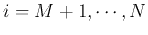
Based on this matrix  , an orthogonal transform of a given signal vector
  can be defined as
The inverse transform is:
Now we consider the variances of the signal components before and after the KLT
transform:
where
 can be considered as the dynamic
energy or information contained in the ith component of the signal, and the trace of
the covariance matrix
can be considered as the dynamic
energy or information contained in the ith component of the signal, and the trace of
the covariance matrix
 represents the total energy
  or
information contained in the signal :
or
information contained in the signal :
Due to the commutativity of trace:
 , we have:
reflecting the fact that the total energy or information of the signal is conserved
after the KLT transform, or any unitary (orthogonal) transform (Parseval's theorem.
However, the energy distribution among all  components can be very different
before and after the KLT transform, as shown below.
components can be very different
before and after the KLT transform, as shown below.
We define the energy contained in the first  components after the transform
 as
as
 is a function of the transform matrix .
Since the total energy is conserved, is also proportional to the
percentage of energy contained in the first
is a function of the transform matrix .
Since the total energy is conserved, is also proportional to the
percentage of energy contained in the first  components.
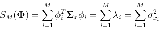
In the following we will show that is maximized if and only if the
transform matrix is the same as that of the KLT:
components.
In the following we will show that is maximized if and only if the
transform matrix is the same as that of the KLT:
In other words, the KLT optimally compacts energy into a few components of the
signal. Consider
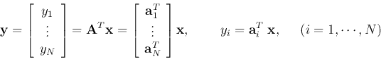
Now we need to find a transform matrix
![${\bf A}=[{\bf a}_1,\cdots,{\bf a}_N]$](img142.png) , so that
, so that
The constraint
 is to guarantee that the column vectors
in are normalized. This constrained optimization problem can be solved
using Lagrange multiplier method by letting the following partial derivative be zero:
is to guarantee that the column vectors
in are normalized. This constrained optimization problem can be solved
using Lagrange multiplier method by letting the following partial derivative be zero:
(* The last equal sign is due to explanation in the
review of linear algebra.)
We see that the column vectors of must be the eigenvectors of  :
:
i.e.,
 has to be an eigen-vector of , and the
transform matrix must be
has to be an eigen-vector of , and the
transform matrix must be
where  's are the orthogonal eigenvectors of corresponding
to eigenvalues
's are the orthogonal eigenvectors of corresponding
to eigenvalues  (
( ):
):
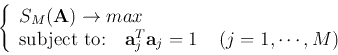
Thus we have proved that the optimal transform is indeed KLT, and
where the ith eigenvalue of is also the average (expectation)
energy contained in the ith component of the signal. If we choose those
 that correspond to the largest eigenvalues of :
 ,
then
,
then
 will be maximized.
Due to KLT's properties of signal decorrelation and energy compaction, it can
be used for data compression by reducing the dimensionality of the data set.
Specifically, we carry out the following steps:
- Find the mean vector
 and the covariance matrix
of the signal vectors .
and the covariance matrix
of the signal vectors .
- Find the eigenvalues ,
 ) of ,
sorted in descending order, and their corresponding eigenvectors
).
) of ,
sorted in descending order, and their corresponding eigenvectors
).
- Choose a lowered dimensionality so that the percentage of energy contained
is no less than a given threshold (e.g., 95%):
- Construct an
 transform matrix composed of the largest eigenvectors
of :
transform matrix composed of the largest eigenvectors
of :
and carry out KLT based on  :
:
As the dimension of  is less than the dimension of , data
compression is achieved for storage or transmission. This is a lossy compression with
the error representing the percentage of information lost:
is less than the dimension of , data
compression is achieved for storage or transmission. This is a lossy compression with
the error representing the percentage of information lost:
 . But as these 's
for
. But as these 's
for
 are the smallest eigenvalues, the error is minimized
(e.g., 5%).
are the smallest eigenvalues, the error is minimized
(e.g., 5%).
- Reconstruct by inverse KLT:
Next: Geometric Interpretation of KLT
Up: klt
Previous: KLT Completely Decorrelates the
Ruye Wang
2016-04-06
![\begin{displaymath}{\bf A}=[{\bf a}_1, \cdots, {\bf a}_{N}],\;\;\;\;\;\;\mbox{or...
...{\bf a}_1^{T} \vdots {\bf a}_{N}^{T} \end{array} \right] \end{displaymath}](img123.png)
![\begin{displaymath}{\bf x}={\bf A}{\bf y}=[{\bf a}_1,\cdots,{\bf a}_{N}]
\left[ ...
...ots y_{N} \end{array} \right]
=\sum_{i=1}^{N} y_i {\bf a}_i \end{displaymath}](img13.png)
![\begin{displaymath}
{\cal E}_x= tr {\bf\Sigma}_x
=\sum_{i=1}^{N} \sigma_{x_i}^2=\sum_{i=1}^{N} E[({x_i}-\mu_{x_i})^2]
=\sum_{i=1}^{N}E(e_{x_i})
\end{displaymath}](img130.png)
![\begin{displaymath}
S_M({\bf A})\stackrel{\triangle}{=}\sum_{i=1}^{M} E\left[(y_...
...right]
=\sum_{i=1}^{M}\sigma_{y_i}^2=\sum_{i=1}^{M}E(e_{y_i})
\end{displaymath}](img134.png)
![$\displaystyle \sum_{i=1}^{M} E(y_i-\mu_{y_1})^2
=\sum_{i=1}^{M} E\left[ {\bf a}_i^{T}({\bf x}-{\bf m}_{x_i})\;({\bf x}-{\bf m}_{x_i})^T{\bf a}_i \right]$](img140.png)
![$\displaystyle \sum_{i=1}^{M} {\bf a}_i^{T}E\left[({\bf x}-{\bf m}_{x_i}) ({\bf ...
...)^T\right] {\bf a}_i^{T}
=\sum_{i=1}^{M} {\bf a}_i^{T} {\bf\Sigma}_x {\bf a}_i$](img141.png)
![$\displaystyle \frac{\partial}{\partial {\bf a}_i}\left[S_M({\bf A})-\sum_{j=1}^...
...j^{T}{\bf\Sigma}_x{\bf a}_j-\lambda_j {\bf a}_j^{T}{\bf a}_j+\lambda_j) \right]$](img145.png)


![\begin{displaymath}
{\bf y}=\left[ \begin{array}{c} y_1 \vdots y_{M} \end{...
...\vdots \vdots x_{N}
\end{array} \right]_{N \times 1}
\end{displaymath}](img162.png)
![\begin{displaymath}{\bf x}=\left[ \begin{array}{c} x_1 \vdots \vdots x_{...
...{c} y_1 \vdots y_{M}
\end{array} \right]_{M \times 1}
\end{displaymath}](img166.png)