Nonlinear Least Squares Regression

The goal of nonlinear least squares (LS) regresion is to model the nonlinear relationship between the dependent variable $y$ and independent variables in ${\bf x}=[x_1,\cdots,x_d]^T$, based on the given training dataset ${\cal D}=\{({\bf x}_n, y_n),\;n=1,\cdots,N\}$, by a nonlinear regression function parameterized by a set of $M$ parameters represented by ${\bf\theta}=[\theta_1,\cdots,\theta_M]^T$:

$$\hat{y}=f(x_1,\cdots,x_d,\;\theta_1,\cdots,\theta_M) =f({\bf x},{\bf\theta})$$ (187)

While the specific form of the nonlinear function is typically determined based on certain prior knowledge, we need to find the parameeter ${\bf\theta}$ for the model to fit the training dataset ${\cal D}$, so that, its output $\hat{\bf y}$ matches the ground truth labeling ${\bf y}$ in the training set, i.e., the residual ${\bf r}={\bf y}-\hat{\bf y}$ is ideally zero:

$${\bf r}({\bf\theta}) =\left[\begin{array}{c}r_1\\ \vdots\\ r_N\en... ... ={\bf y}-\hat{\bf y}({\bf\theta}) ={\bf y}-{\bf f}({\bf X},{\bf\theta})={\bf0}$$ (188)

where $\hat{y}({\bf x}_n,{\bf\theta})=f_n({\bf\theta})=f({\bf x}_n,{\bf\theta})$ is the predicted output by the regression function based on the nth data point ${\bf x}_n$. We see that the regression problem is equivalent to solving a nonlinear equation system of $N$ equations for the $M$ unknown parameters in ${\bf\theta}$. As typically there are many more data samples than the unknown parameters, i.e., $N\gg M$, the equation ${\bf r}={\bf0}$ is over-overconstrained without an exact solution. We therefore consider the the optimal parameter ${\bf\theta}^*$ that minimizes the sum-of-squared error based on the residual ${\bf r}$:

$$\varepsilon({\bf\theta})=\frac{1}{2}\vert\vert{\bf r}\vert\vert^2 =\frac{1}{2}\sum_{n=1}^N r_n^2 =\frac{1}{2}\sum_{n=1}^N[y_n-f_n({\bf\theta})]^2$$ (189)

To do so, we first consider the gradient descent method based on the gradient of this error function:

$${\bf g}_\varepsilon({\bf\theta}) = \frac{d}{d{\bf\theta}}\varepsilon({\bf\theta}) =\frac{d}{d{\bf\th... ...c{1}{2}\sum_{n=1}^N r_n^2\right) =\sum_{n=1}^N \frac{d\,r_n}{d{\bf\theta}}\;r_n$$

$$= -\sum_{n=1}^N \frac{d}{d{\bf\theta}} f_n({\bf\theta}) [y_n-f_n({\bf\theta})] =-{\bf J}_f^T\;{\bf r}$$ (190)

where ${\bf J}_f$ is the $N\times M$ Jacobian matrix ${\bf J}_f$ of ${\bf f}({\bf X},{\bf\theta})$. The mth component of the gradient vector is

$$g_m({\bf\theta}) = \frac{\partial}{\partial\theta_m}\varepsilon({\bf\theta}) =\frac{... ...\partial\theta_m}r_n^2 =\sum_{n=1}^N \frac{\partial r_n}{\partial\theta_m}\;r_n$$

$$= \sum_{n=1}^N \frac{\partial f_n({\bf\theta})}{\partial\theta_m} [... ...,[f_n({\bf\theta})-y_n] \sum_{n=1}^N J_{nm}\,r_n \;\;\;\;\;\;\;\;(m=1,\cdots,M)$$ (191)

where $J_{nm}=\partial\,f_n({\bf\theta})/\partial\theta_m$ is the element in the nth row and mth column of ${\bf J}_f$, which is simply the negative version of Jacobian of ${\bf r}={\bf y}-{\bf f}({\bf X},{\bf\theta})$:

$${\bf J}_r({\bf\theta})=\frac{d}{d{\bf\theta}}{\bf r}({\bf\theta})... ... =-\frac{d}{d{\bf\theta}} {\bf f}({\bf X},{\bf\theta}) =-{\bf J}_f({\bf\theta})$$ (192)

The optimal parameters in ${\bf\theta}$ that minimizes $\varepsilon({\bf\theta})$ can now be found iteratively by the gradient descent method:

$${\bf\theta}_{n+1}={\bf\theta}_n-\delta_n {\bf g}_\varepsilon({\bf\theta}_n) ={\bf\theta}_n-\delta_n {\bf J}_f^T\;{\bf r}$$ (193)

Setting the value for the step size $\delta_n$ properly may be tricky, as it depends on the specific landscape of the error hypersurface $\varepsilon({\bf\theta})$. If $\delta_n$ is too large, a minimum may be skipped over, but if $\delta_n$ is too large, the convergence of the iteration may be too slow.

This gradient method is also called batch gradient descent (BGD), as the gradient in Eq. (190) is calculated based on the entire batch of all $N$ data points in the dataset ${\cal D}$ in each iteration. When the size of the dataset is large, BGD may be slow due to the high computational complexity. In this case the method of stochastic gradient descent (SGD) can be used, which approximates the gradient based on only one of the $N$ data points uniformly randomly chosen from the dataset in each iteration, i.e., the summation in Eq. (190) contains only one term corresponding to the chosen sample ${\bf x}_n$:

$${\bf g}_n({\bf\theta})=\frac{d}{d{\bf\theta}} \frac{1}{2} r_n^2 =r_n\frac{d\,r_n}{d{\bf\theta}}$$ (194)

The expectation of ${\bf g}_n$ based on one data point is the same as the true gradient (scaled by $1/N$) based on all $N$ data points in the dataset

$$E[ {\bf g}_n({\bf\theta}) ] =\sum_{n=1}^N P({\bf x}_n) {\bf g}_n(... ...{N}\sum_{n=1}^N \frac{dr_n}{d{\bf\theta}}\;r_n =\frac{1}{N}{\bf g}({\bf\theta})$$ (195)

As the data are typically noisy, the SGD gradient based on only one data point may be in a direction very different from the true gradient based on the mean of all $N$ data points, and the resulting search path in the M-D space may be in a very jagged zig-zag shape, and the iteration may converge slowly. However, as the computational complexity in each iteration is much reduced, we can afford to carry out a large number of iterations with an overall search path generally coinciding with that of the BGD method.

Some trade-off between BGD and SGD can be made so that the gradient is estimated based on more than one but less than all $N$ data points in the dataset, the resulting method, called mini-batch gradient descent, can take advantage of both methods. The methods of stochastic and mini-batch gradient descent are widely used in machine learning, such as in the method of artificial neural networks, which can be treated as a nonlinear regression problem, considered in a later chapter.

Alternatively, the optimal parameter ${\bf\theta}^*$ of the nonlinear regression function $f({\bf x},{\bf\theta})$ can also be found by the Gauss-Newton method, which directly solves the nonlinear over-determined equation system ${\bf r}({\bf\theta})={\bf y}-{\bf f}({\bf X},{\bf\theta})={\bf0}$ in Eq. (188), based on the iterative Newton-Raphson method in Eq. () in Chapter 2:

$${\bf\theta}_{n+1} ={\bf\theta}_n-{\bf J}_r^-\;{\bf r} ={\bf\theta... ... J}_r^T\;{\bf r} ={\bf\theta}_n+({\bf J}_f^T{\bf J}_f)^{-1}{\bf J}_f^T\;{\bf r}$$ (196)

The last equality is due to the fact that ${\bf J}_r=-{\bf J}_f$. Here ${\bf J}_f^T{\bf J}_f$ in the pseudo-inverse is actually an approximation of the Hessian ${\bf H}_\varepsilon$ of the error function $\varepsilon({\bf\theta})$, as shown in the example in a previous chapter, and $-{\bf J}^T_f{\bf r}={\bf g}_\varepsilon({\bf\theta})$ is the gradient of the error function given in Eq. (190). So the iteration above is essentially:

$${\bf\theta}_{n+1} ={\bf\theta}_n-{\bf J}_r^-\;{\bf r} \approx {\b... ...a}_n -{\bf H}_\varepsilon^{-1}({\bf\theta}_n){\bf g}_\varepsilon({\bf\theta}_n)$$ (197)

same as the Newton-Raphson method based on the second order Hessian as well as the first oder gradient. We therefore see that the Gauss-Newton method is actually for minimizing the sum-of-squares error is essentially the same as the Newton-Raphson method, with the only difference that the Hessian ${\bf H}_\varepsilon \approx {\bf J}_f^T{\bf J}_f$ as the second order derivative of the error function $\varepsilon({\bf\theta})$ is approximated by the Jacobian ${\bf J}_f{\bf\theta}$ as the first order derivative of the regression function ${\bf f}({\bf x},{\bf\theta})$, making the implementation computationally easier.

In the special case of linear regression function ${\bf f}({\bf w})={\bf x}^T{\bf w}$, we have:

$$\hat{\bf y}={\bf f}({\bf X},{\bf w}) =\left[\begin{array}{c}f({\b... ...nd{array}\right]{\bf w} =[{\bf x}_1,\cdots,{\bf x}_N]^T{\bf w}={\bf X}^T{\bf w}$$ (198)

where ${\bf w}=[w_0,\,w_1,\cdots,w_d]^T$ and ${\bf x}_i=[1, x_{i1},\cdots,x_{id}]^T$ are both augmented $d+1$ dimensional vectors and ${\bf X}=[{\bf x}_1,\cdots,{\bf x}_N]$. The Taylor series is

$$f({\bf X},{\bf w}+\Delta{\bf w})={\bf X}^T({\bf w}+\Delta{\bf w}) ={\bf X}^T{\bf w}+{\bf X}^T\Delta{\bf w}$$ (199)

and the Jacobian is

$${\bf J}_f({\bf w})={\bf X}^T$$ (200)

Now Eq. (196) becomes

$${\bf w}_{n+1} = {\bf w}_n+({\bf X}^T)^-({\bf y}-{\bf X}^T{\bf w}_n) ={\bf w}_n+({\bf X}{\bf X}^T)^{-1}{\bf X}({\bf y}-{\bf X}^T{\bf w}_n)$$

$$= {\bf w}_n+({\bf X}{\bf X}^T)^{-1}{\bf X}{\bf y} -({\bf X}{\bf X}^T)^{-1}({\bf X}{\bf X}^T){\bf w}_n$$

$$= ({\bf X}{\bf X}^T)^{-1}{\bf X}{\bf y}=({\bf X}^T)^-{\bf y}$$ (201)

i.e., the optimal parameter ${\bf w}^*$ can be found in a single step without iteration, same as that in Eq. (116).

The Matlab code for the essential parts of the algorithm is listed below, where data(:,1) and data(:,2) are the observed data containing $N$ samples $x_1,\cdots,x_N$ in the first column and their corresponding function values $y_1,\cdots,y_N$ in the second column. In the code segment below, the regression function (e.g., an exponential model) is symbolically defined, and then a function NLregression is called to estimate the function parameters:

    sym x;                            % symbolic variables
    a=sym('a',[3 1]);                 % symbolic parameters
    f=@(x,a)a(1)*exp(a(2)*x)+a(3)|    % symbolic function
    [a er]=NLregression(data(:,1),data(:,2),f,3);  % call regression

The code below estimates the $M$ parameters of the regression function based on Newton's method.

    function [a er]=NLregression(x,y,f,M)   % nonlinear regression
        N=length(x);                  % number of data samples
        a=sym('a',[M 1]);             % M symbolic parameters 
        F=[];                     
        for i=1:N
            F=[F; f(x(i),a)];         % evaluate function at N given data points
        end
        J=jacobian(F,a);              % symbolic Jacobian 
        J=matlabFunction(J);          % convert to a true function
        F=matlabFunction(F);          
        a1=ones(M,1);                 % initial guesses for M parameters 
        n=0;                          % iteration index             
        da=1;
        while da>tol                  % terminate if no progress made
            n=n+1;
            a0=a1;                    % update parameters
            J0=J(a0(1),a0(2));        % evaluate Jacobian based on a0
            Jinv=pinv(J0);            % pseudo inverse of Jacobian
            r=y-F(a0(1),a0(2));       % residual
            a1=a0+Jinv*r;             % Newton iteration 
            er=norm(r);               % residual error
            da=norm(a0-a1);           % progress
        end
    end

where tol is a small value for tollerance, such as $10^{-6}$.

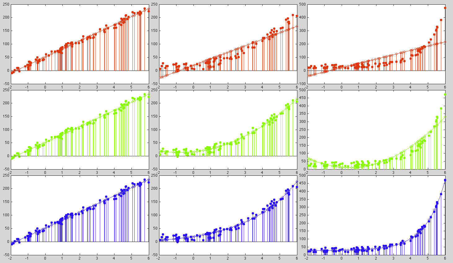
Example 1

Consider three sets of data (shown as the solid dots in the three columns in the plots below) are fitted by three different models (shown as the open circles in the plots):

1. Linear model: $y=f_1(x)=ax+b$
2. quadratic model: $y=f_2(x)=ax^2+bx+c$
3. Exponential model: $y=f_3(x)=a\,e^{bx}+c$

These are the parameters for the three models to fit each of the three datasets:

$$\begin{array}{r\vert\vert r\vert\vert r\vert r\vert r\vert\ve... ...del\;3: & 2.197 & 0.885 & 27.241 & 8.3393 \\ \hline \end{array}$$

We see that the first dataset can be fitted by all three models equally well with similar error (when $a\approx 0$ in model 2, it is approximately a linear functions), the second dataset can be well fitted by either the second or the third model, while the third dataset can only be fitted by the third exponential model.

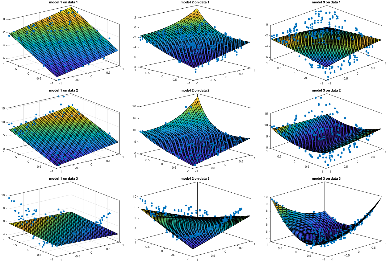
Example 2

Based on the following three functions with four parameters $a=1,\;b=2,\;c=3,\;d=4$, three sets of 2-D data points are generated (with some random noise added), shown in the figure below as the dots in the three rows.

$$f_1({\bf x}) = ax_1+bx_2-c$$

$$f_2({\bf x}) = \exp(ax_1+bx_2)-cx_1x_2+d$$

$$f_3({\bf x}) = ax_1^2-bx_1x_2+cx_2^2+d$$ (202)

Then each of three datasets are fitted by the three functions as models while the optimal parameters are found by the Gauss-Newton method.

$$\begin{array}{r\vert\vert r\vert\vert r\vert r\vert r\vert r\... ...el\;3: & 0.94 & 2.05 & 2.99 & 4.02 & 4.09 \\ \hline \end{array}$$

The Levenberg-Marquardt algorithm (LMA) or damped least-squares method is a method widely used to minimize a sum-of-squares error $\varepsilon$ as in Eq. (189). The LMA is an interpolation or trade-off between the the gradient descent method based on the first order derivative of the error function to be minimized, and the Gauss-Newton method based on both the first and second order derivatives of the error function, both discussed above. As the LMA can take advantage of both methods and is therefore more robust. Even if the initial guess is far from the solution corresponding to the minimum of the objective function, the iteration can still converge toward the solution.

Specifically, the LMA modifies Eq. (196)

$${\bf\theta}_{n+1}={\bf\theta}_n +{\bf J}^-_f({\bf\theta}_n)[ {\bf... ...\bf J}_n^T{\bf J}_n)^{-1}{\bf J}_n^T [ {\bf y}-{\bf f}({\bf X},{\bf\theta}_n) ]$$ (203)

to include an extra term proportional to the identity matrix ${\bf I}$:

$${\bf\theta}_{n+1}={\bf\theta}_n +({\bf J}_n^T{\bf J}_n+\lambda{\bf I})^{-1}{\bf J}_n^T [ {\bf y}-{\bf f}({\bf X},{\bf\theta}_n) ]$$ (204)

where $\lambda\ge 0$ is the non-negative damping factor, which is to be adjusted at each iteration. We recognize that this is actaully similar to Eq. (144) for ridge regression.

In each iterative step, if $\lambda$ is small and the error function $\varepsilon({\bf\theta}_n)$ decreases quickly, indicating the Gauss-Newton is effective in the sense that the error fucntion is well modeled as a quadratic function by the first and second order terms of the Taylor series, we will keep $\lambda$ small. On the other hand, if $\varepsilon$ decreases slowly, indicating the error function may not be well modeled as a quadratic function, due possibly to the fact that the current ${\bf\theta}_n$ is far away from the minimum, then we let $\lambda$ take a large value, so that the term ${\bf J}_n^T{\bf J}_n$ becomes insignificant, and Eq. (204) approaches

$${\bf\theta}_{n+1} ={\bf\theta}_n+\lambda {\bf J}^T_n ({\bf y}-{\bf f}({\bf\theta})) ={\bf\theta}_n-\alpha {\bf g}_\varepsilon({\bf\theta})$$ (205)

Now ${\bf\theta}_n$ is updated along the negative direction of the gradient in Eq. (190):

$${\bf g}_\varepsilon({\bf\theta}) \propto {\bf J}^T ({\bf f}({\bf\theta})-{\bf y})$$ (206)

with some step size $\alpha$.

By adjusting the parameter $\lambda$, the LMA can switch between either of the two methods for the same purpose of minimizing $\varepsilon({\bf\theta})$. When the value of $\lambda$ is small, the iteration is dominated by the Gauss-Newton method that approximate the error function by a quadratic function based on the second order derivatives. If the error reduces slowly, indicating the error function cannot be approximated by a quadratic function, a greater value of $\lambda$ is used to switch to the gradient descent method.