Bayesian Linear Regression

We revisit the linear regression problem but from the viewpoint of Bayesian inference. Now the parameter ${\bf w}$ in the linear regression model $\hat{y}=f({\bf x},{\bf w})={\bf x}^T{\bf w}$ is assumed to be a random vector, and, as a function of ${\bf w}$, the regression function $f({\bf x},{\bf w})$ is also random, and so is the residual based on the training set ${\cal D}=\{ {\bf X},{\bf y}\}$:

$${\bf r}={\bf y}-\hat{\bf y}={\bf y}-{\bf X}^T{\bf w}, \;\;\;\;\;\;\;\;\; \;\;\;\;\;\;\;\;\; {\bf y}=\hat{\bf y}+{\bf r}={\bf f}({\bf X})+{\bf r} ={\bf X}^T{\bf w}+{\bf r}$$ (157)

We further assume ${\bf w}$ has a zero-mean normal prior pdf:

$$p({\bf w})={\cal N}({\bf w},\,{\bf0},\,{\bf\Sigma}_w) \propto \exp\left( -\frac{1}{2}{\bf w}^T{\bf\Sigma}_w^{-1}{\bf w}\right),$$ (158)

based on the desire that the weights in ${\bf w}$ should take values around zero, instead of large values on either positive or negative, to avoid potiential overfitting. We also assume the residual ${\bf r}$ has a zero-mean normal pdf with a diagonal covariance matrix, i.e., all components of ${\bf r}$ are indepenent of each other:

$$p({\bf r})={\cal N}({\bf r},\,{\bf0},\,\sigma_r^2{\bf I}) \propto... ... r}\right) =\exp\left(-\frac{\vert\vert{\bf r}\vert\vert^2}{2\sigma_r^2}\right)$$ (159)

As a linear transformation of ${\bf w}$, the regression function $\hat{\bf y}={\bf X}^T{\bf w}$ also has a zero-mean Gaussian distribution, and so is ${\bf y}={\bf X}^T{\bf w}+{\bf r}$ as the sum of two Gaussians.

To obtain the model parameter ${\bf w}$, we consider its likelihood $L({\bf w}\vert{\cal D})$ based on the observed data ${\cal D}=\{ {\bf X},{\bf y}\}$:

$$L({\bf w}\vert{\cal D}) \propto p({\cal D}\vert{\bf w})=p({\bf y}\vert{\bf X},{\bf w}) =p({\bf X}^T{\bf w} +{\bf r})={\cal N}({\bf y},{\bf X}^T{\bf w},\sigma_r^2{\bf I})$$

$$\propto \exp\left( -\frac{1}{2\sigma_r^2} ({\bf y}-{\bf X}^T{\bf w})^T({\... ...})\right) =\exp\left(-\frac{1}{2\sigma_r^2}\vert\vert{\bf r}\vert\vert^2\right)$$ (160)

This is the same Gaussian as $p({\bf r})={\cal N}({\bf r},{\bf0},\sigma_r^2{\bf I})$, but shifted by ${\bf X}^T{\bf w}$. Now we can find the optimal model parameter ${\bf w}^*$ by maximizing the likelihood $L({\bf w}\vert{\cal D})$. This method is called maximum likelihood estimation (MLE). But as maximizing $L({\bf w}\vert{\cal D})$ is equivalent to minimizing the SSE $\vert\vert{\bf r}\vert\vert^2$, the MLE method is equivalent to the least squares method considered before.

Maximizing the likelihood above is equivalent to minimizing the negative log likelihood:

$$-l({\bf w}\vert {\bf X},{\bf y})=-\log L({\bf w}\vert {\bf X},{\b... ...ert\vert{\bf r}\vert\vert^2}{2\sigma_r^2} \propto \vert\vert{\bf r}\vert\vert^2$$ (161)

which is the same as the squared error $\varepsilon({\bf w})$ defined in Eq. (114) to be minimized by the LS method previously considered. We therefore see that the least squares method and the maximum likelihood method are equivalent to each other in this case.

We can further find the posterior $p({\bf w}\vert{\cal D})$ of the model parameter ${\bf w}$ given the observed data ${\cal D}$, as the product of prior $p({\bf w})$ and likelihood $L({\bf w}\vert{\cal D})\propto p({\bf y}\vert{\bf X},{\bf w})$:

$$p({\bf w}\vert{\cal D}) = p({\bf w}\vert{\bf X},{\bf y}) =\frac{p({\cal D}\vert{\bf w})\,p(... ...})} =\frac{p({\bf y}\vert{\bf X},{\bf w})\; p({\bf w})}{p({\bf y}\vert{\bf X})}$$

$$\propto p({\bf y}\vert{\bf X},{\bf w})\;p({\bf w}) ={\cal N}({\bf y},{\bf X}^T{\bf w},\sigma_r^2{\bf I})\; {\cal N}({\bf w},{\bf0},{\bf\Sigma}_w)$$

$$\propto \exp\left[-\frac{1}{2}\left(\frac{1}{\sigma_r^2}({\bf y}-{\bf X}^... ...)^T({\bf y}-{\bf X}^T{\bf w})+{\bf w}^T{\bf\Sigma}_w^{-1} {\bf w}\right)\right]$$

$$\propto \exp\left[-\frac{1}{2}\left(\frac{1}{\sigma_r^2}{\bf y}^T{\bf y} ... ...2}{\bf w}^T{\bf XX}^T{\bf w} +{\bf w}^T{\bf\Sigma}_w^{-1} {\bf w}\right)\right]$$

$$\propto \exp\left[-\frac{1}{2}\left({\bf w}^T \left(\frac{1}{\sigma_r^2}{... ...ma}_w^{-1}\right){\bf w} -\frac{2}{\sigma_r^2}({\bf Xy})^T{\bf w}\right)\right]$$ (162)

where all constant scaling factors (irrelavant to ${\bf w}$) are dropped for simplicity. As both the prior and the likelihood are Gaussian, this this posterior, when normalized, is also Gaussian in terms of the mean ${\bf m}_{w/d}$ and covariance ${\bf\Sigma}_{w/d}$:

$$p({\bf w}\vert{\cal D}) ={\cal N}({\bf w},{\bf m}_{w/d},{\bf\Sigma}_{w/d} ) \propto \exp \left[ -\frac{1}{2} \left( ({\bf w}-{\bf m}_{w/d})^T {\bf\Sigma}_{w/d}^{-1}({\bf w}-{\bf m}_{w/d}) \right) \right]$$

$$\propto \exp \left[ -\frac{1}{2} \left( {\bf w}^T{\bf\Sigma}_{w/d}^{-1}{\bf w}-2{\bf m}_{w/d}^T {\bf\Sigma}_{w/d}^{-1}{\bf w} \right) \right]$$ (163)

with the following covariance and mean:

$${\bf\Sigma}_{w/d} = \left(\frac{1}{\sigma_r^2}{\bf X}{\bf X}^T+{\bf\Sigma}_w^{-1}\right)^{-1}$$

$${\bf m}_{w/d} = \frac{1}{\sigma_r^2}{\bf\Sigma}_{w/d} {\bf Xy} =\left({\bf X}{\bf X}^T+\sigma_r^2{\bf\Sigma}_w^{-1}\right)^{-1} {\bf Xy}$$ (164)

Now we can find the optimal model parameter ${\bf w}^*={\bf m}_{w/d}$ equal to the mean of the Gaussian posterior where it is maximized. This solution is called the maximum a posteriori (MAP) estimate of the model parameter ${\bf w}$.

We can now predict the function value of any unlabeled test data point ${\bf x}_*$ based on the conditional probability distribution $p(f_*\vert{\bf x}_*,{\cal D})$ of the regression model $\hat{y}_*=f_*=f({\bf x}_*)={\bf x}_*^T{\bf w}$, which, as a linear transformation of the random parameters in ${\bf w}$, is also Gaussian (see properties of Gaussians):

$$p(f_*\vert{\bf x}_*,{\cal D}) = p({\bf x}^T_*{\bf w}\vert{\bf x}_... ...\cal N}(f_*,{\bf x}_*^T{\bf m}_{w/d}, \;{\bf x}_*^T{\bf\Sigma}_{w/d} {\bf x}_*)$$ (165)

with the following mean and variance:

$$\E[f_*\vert{\bf x}_*,{\bf X},{\bf y}] = {\bf x}_*^T{\bf m}_{w/d} ={\bf x}_*^T \left({\bf X}{\bf X}^T+\sigma_r^2{\bf\Sigma}_w^{-1}\right)^{-1}{\bf Xy}$$ (166)

$$\Var[f_*\vert{\bf x}_*,{\bf X},{\bf y}] = {\bf x}_*^T{\bf\Sigma}_{w/d} {\bf x}_* ={\bf x}_*^T\left(\frac{1}{\sigma_r^2}{\bf X}{\bf X}^T +{\bf\Sigma}_w^{-1}\right)^{-1}{\bf x}_*$$ (167)

Furthermore, given a set of $M$ unlabeled test data points in ${\bf X}_*=[{\bf x}_{1*},\cdots,{\bf x}_{M*}]^T$, we can find

$$\hat{\bf y}_*={\bf f}_*={\bf f}({\bf x}_*) =\left[\begin{array}{c... ...}\right]{\bf w} =[{\bf x}_{1*},\cdots,{\bf x}_{M*}]^T{\bf w}={\bf X}^T_*{\bf w}$$ (168)

As a linear combination of Guassian ${\bf w}$, ${\bf f}_*={\bf X}_*^T{\bf w}$ is also Gaussian:

$$p({\bf f}_*\vert{\bf X}_*,{\cal D})=p({\bf f}_*\vert{\bf X}_*,{\b... ... N}({\bf f}_*,{\bf X}^T_*{\bf m}_{w/d},\;{\bf X}^T_*{\bf\Sigma}_{w/d}{\bf X}_*)$$ (169)

with the following mean and covariance:

$$\E[ {\bf f}_*\vert{\bf X}_*,{\bf X},{\bf y} ] = \E[ {\bf X}^T_*{\bf w} ]={\bf X}^T_*\E[ {\bf w} ]={\bf X}^T_*{\bf... ...f X}^T_*\left({\bf X}{\bf X}^T+\sigma_r^2{\bf\Sigma}_w^{-1}\right)^{-1}{\bf Xy}$$ (170)

$$Cov({\bf f}_*\vert{\bf X}_*,{\bf X},{\bf y}) = \E[{\bf f}_*{\bf f}_*^T] =\E[ {\bf X}^T_*{\bf w} {\bf w}^T{\bf X}... ...f X}^T_*\E[ {\bf w} {\bf w}^T] {\bf X}_* ={\bf X}^T_*{\bf\Sigma}_{w/d}{\bf X}_*$$ (171)

The mean $\E[{\bf f}_*\vert{\bf X}_*,{\bf X},{\bf y} ]$ above can be considered as the estimated function value $\hat{\bf y}_*={\bf f}_*={\bf X}_*^T{\bf w}$ at the test points in ${\bf X}_*$, while the variance $\Var[{\bf f}_*\vert{\bf X}_*,{\bf X},{\bf y}]$ as the confidence or certainty of the estimation.

Such a result produced by the Bayesian method in terms of the mean and covariance of ${\bf f}_*=\hat{\bf y}_*$ as a random vector is quite different from the result produced by a frequentist method such as the linear least square regression in terms of an estimated value of $\hat{\bf y}_*$ as a deterministic variable. However, in the special case of $\sigma_r=0$, i.e., the residual ${\bf r}$ is no longer treated as a random variable, then Eq. (170) above becomes the same as Eq. (117) produced by linear least square regression, in other words, the linear method method can be considered as a special case of the Bayesian regression when the residual is deterministic.

The method considered above is based on the linear regression model $f({\bf x})={\bf x}^T{\bf w}$, but it can also be generalized to nonlinear functions, same as in the case of generalized linear regression discussed previously. To do so, the regression function is assumed to be a linear combination of a set of $K$ nonlinear mapping functions $\varphi_k({\bf x})\;(k=1,\cdots,K)$:

$$y=f({\bf x})+e=\sum_{k=1}^K w_k \,\varphi_k({\bf x})+r ={\bf w}^T {\bf\phi}({\bf x})+r={\bf\phi}^T({\bf x}){\bf w}+r$$ (172)

where

$${\bf w}=[w_1,\cdots,w_K]^T,\;\;\;\;\;\; {\bf\phi}({\bf x})=[\varphi_1({\bf x}),\cdots,\varphi_K({\bf x})]^T$$ (173)

For example, some commenly used mapping functions are listed in Eq. (155).

Applying this regression model to each of the $N$ observed data points in ${\cal D}=\{({\bf x}_n,y_n),\;(n=1,\cdots,N)\}$, we get $\hat{y}_n=\sum_{k=1}^K w_k \,\varphi_k(x_n)$ with residual $r_n=y_n-\hat{y}_n$, which can be written in matrix form:

$${\bf y} = \left[\begin{array}{c}y_1\\ \vdots\\ y_N\end{array}\right]_{N\tim... ...imes 1} +\left[\begin{array}{c}r_1\\ \vdots\\ r_N\end{array}\right]_{N\times 1}$$

$$= \left[\begin{array}{c} {\bf\phi}^T_1\\ \vdots\\ {\bf\phi}^T_N \end{array}\right]{\bf w}+{\bf r}={\bf\Phi}^T{\bf w}+{\bf r}$$ (174)

where, as previously defined in Eq. (152),

$${\bf\phi}_n={\bf\phi}({\bf x}_n)=\left[\begin{array}{c} \varphi_1... ..._n) \end{array}\right], \;\;\;\;\;\; {\bf\Phi}=[{\bf\phi}_1,\cdots,{\bf\phi}_N]$$ (175)

As this nonlinear model $\hat{\bf y}={\bf\Phi}^T{\bf w}$ is in the same form as the linear model $\hat{\bf y}={\bf X}^T{\bf w}$, all previous discussion for the linear Bayesian regression is still valid for this nonlinear model, if ${\bf X}=[{\bf x}_1,\cdots,{\bf x}_N]_{(d+1)\times N}$ is replaced by ${\bf\Phi}=[{\bf\phi}_1,\cdots,{\bf\phi}_N]_{K\times N}$. We can get the covariance matrix and mean vector of the posterior $p({\bf w}\vert{\cal D})$ in the K-dimensional space based on the observed data ${\cal D}=\{ {\bf X},{\bf y}\}$:

$${\bf\Sigma}_{w/d} = \left(\frac{1}{\sigma_r^2}{\bf\Phi}{\bf\Phi}^T +{\bf\Sigma}_w^{-1}\right)^{-1}$$

$${\bf m}_{w/d} = \frac{1}{\sigma_r^2}{\bf\Sigma}_{w/d}{\bf\Phi}{\bf y} =\left({\bf\Phi}{\bf\Phi}^T+\sigma_r^2{\bf\Sigma}_w^{-1}\right)^{-1} {\bf\Phi}{\bf y}$$ (176)

The function $\hat{\bf y}_*={\bf f}({\bf X}_*)$ of the multiple test points in ${\bf X}_*=[{\bf x}_{*1},\cdots,{\bf x}_{*M}]^T$ is a linear transformation of ${\bf w}$:

$$\hat{\bf y}_*={\bf f}_*={\bf f}({\bf x}_*) =\left[\begin{array}{c... ...ight]_*{\bf w} =[{\bf\phi}_1,\cdots,{\bf\phi}_M]^T{\bf w} ={\bf\Phi}^T_*{\bf w}$$ (177)

and it also has a Gaussian joint distribution:

$$p({\bf f}_*\vert{\bf X}_*,{\bf X},{\bf y})={\cal N}({\bf\Phi}^T_*{\bf m}_{w/d}, \; {\bf\Phi}^T_*{\bf\Sigma}_{w/d}{\bf\Phi}_*)$$ (178)

with the mean and covariance:

$$\E[ {\bf f}_*\vert{\bf X}_*,{\bf X},{\bf y} ] = \E[ {\bf\Phi}^T_*{\bf w} ]={\bf\Phi}^T_*\E[ {\bf w} ] ={\bf\Phi}^T_*{\bf m}_{w/d}$$

$$Cov({\bf f}_*\vert{\bf X}_*,{\bf X},{\bf y}) = \E[ {\bf f}_*{\bf f}_*^T ] =\E[ {\bf\Phi}^T_*{\bf w} {\bf w}^T{\b... ...*\E[ {\bf w} {\bf w}^T ] {\bf\Phi}_* ={\bf\Phi}^T_*{\bf\Sigma}_{w/d}{\bf\Phi}_*$$ (179)

They can be reformulated to become:

$$\E[ {\bf f}_*\vert{\bf X}_*,{\bf X},{\bf y} ] = {\bf\Phi}^T_*{\bf m}_{w/d} ={\bf\Phi}^T_* \left({\bf\Phi}{\bf\Phi}^T+\sigma_r^2{\bf\Sigma}_w^{-1}\right)^{-1} {\bf\Phi}{\bf y}$$

$$= {\bf\Phi}^T_* ({\bf\Sigma}_w{\bf\Phi}) ({\bf\Sigma}_w{\bf\Phi})^{... ...bf\Phi}^T+\sigma_r^2{\bf\Sigma}_w^{-1}\right)^{-1} ({\bf\Phi}^{-1})^{-1}{\bf y}$$

$$= {\bf\Phi}^T_*{\bf\Sigma}_w{\bf\Phi} \left[{\bf\Phi}^{-1}\left({\b... ...+\sigma_r^2{\bf\Sigma}_w^{-1}\right){\bf\Sigma}_w{\bf\Phi} \right]^{-1} {\bf y}$$

$$= {\bf\Phi}^T_*{\bf\Sigma}_w{\bf\Phi}({\bf\Phi}^T{\bf\Sigma}_w{\bf\Phi} +\sigma_r^2{\bf I})^{-1}{\bf y}$$ (180)

and

$$Cov({\bf f}_*\vert{\bf X}_*,{\bf X},{\bf y}) = {\bf\Phi}^T_*{\bf\Sigma}_{w/d}{\bf\Phi}_* ={\bf\Phi}^T_*\left(\frac{1}{\sigma_r^2}{\bf\Phi}{\bf\Phi}^T +{\bf\Sigma}_w^{-1}\right)^{-1}{\bf\Phi}_*$$

$$= {\bf\Phi}^T_*\left[{\bf\Sigma}_w-{\bf\Sigma}_w{\bf\Phi} ({\bf\Phi... ...a}_w{\bf\Phi}+\sigma_r^2{\bf I})^{-1}{\bf\Phi}^T{\bf\Sigma}_w\right]{\bf\Phi}_*$$

$$= {\bf\Phi}^T_*{\bf\Sigma}_w{\bf\Phi}_*-{\bf\Phi}_*^T{\bf\Sigma}_w{... ...bf\Sigma}_w{\bf\Phi}+\sigma_r^2{\bf I})^{-1}{\bf\Phi}^T{\bf\Sigma}_w{\bf\Phi}_*$$ (181)

where we have used Theorem 1 in the Appendices.

We note that in these expressions the mapping function $\varphi({\bf x})$ only shows up in the quadratic form of ${\bf\Phi}^T{\bf\Sigma}_w{\bf\Phi}$, ${\bf\Phi}^T{\bf\Sigma}_w{\bf\Phi}_*$, or ${\bf\Phi}^T_*{\bf\Sigma}_w{\bf\Phi}_*$. This suggests that we may consider using kernel method, by which some significant advantage may be gained (such as in the support-vector machines). Specifically, if we replace the mn-th component ${\bf\phi}^T({\bf x}_m){\bf\Sigma}_w{\bf\phi}({\bf x}_n)$ of ${\bf\Phi}^T{\bf\Sigma}_w{\bf\Phi}$ by a kernel function only in terms of ${\bf x}_m$ and ${\bf x}_n$:

$${\bf\phi}^T({\bf x}_m){\bf\Sigma}_w{\bf\phi}({\bf x}_n)=k({\bf x}_m,{\bf x}_n) =k({\bf x}_n,{\bf x}_m)$$ (182)

then the mapping function $\varphi({\bf x})$ no longer needs to be explicitly specified. This idea is called the kernel trick, Now we have

$${\bf\Phi}^T{\bf\Sigma}_w{\bf\Phi} =\left[\begin{array}{c}{\bf\phi... ...k({\bf x}_N,{\bf x}_1)&\cdots&k({\bf x}_N,{\bf x}_N)\end{array}\right] ={\bf K}$$ (183)

and similarly we also have ${\bf\Phi}^T{\bf\Sigma}_w{\bf\Phi}_*={\bf K}_*$ and ${\bf\Phi}_*^T{\bf\Sigma}_w{\bf\Phi}={\bf K}_*^T$. These kernel functions are symmetric, same as all covariance matrices. Now the mean and covariance of ${\bf f}_*$ given above can be expressed as:

$$\E[ {\bf f}_*] = {\bf K}_*^T\left({\bf K}+\sigma_r^2{\bf I}\right)^{-1}{\bf y}$$

$$Cov({\bf f}_*) = {\bf K}_{**}-{\bf K}_*^T \left({\bf K}+\sigma_r^2{\bf I}\right)^{-1} {\bf K}_*$$ (184)

As a general summary of the method discussed above, we note that it is essentially different from the frequentist approach, in the sense that the estimated result produced is no longer a set specific values of some unknown variables in question (function values, parameters of regression models, etc.), but the probability distribution of these variables in terms of the expectation and covariance. Consequently, we can not only treat the expectation as the estimated values, but also use the variance as the confidence or certainty of such an estimation.

Below is a segment of Matlab code for estimating the mean and covariance of weight vector ${\bf w}$ by the Bayes linear regression. Here X and y are for ${\bf X}$ and ${\bf y}$ of the training data ${\cal D}$, and Xstar, Phi and Phistar are for ${\bf X}_*$, ${\bf\Phi}$ and ${\bf\Phi}_*$, respectively.

    SigmaP=eye(d);                  % prior variance of r in original space
    SigmaQ=eye(D);                  % prior variance of r in feature space
    Sigmaw1=inv(X*X'/sigmaN^2+inv(SigmaP));        % covariance of w by Bayes regression
    Sigmaw2=inv(Phi0*Phi0'/sigmaN^2+inv(SigmaQ));  % covariance of w with basis function
       
    w0=inv(X*X')*X*y                % weight vector w by LS method
    w1=Sigmaw1*X*y/sigmaN^2         % mean of w by Bayes regression
    w2=Sigmaw2*Phi0*y/sigmaN^2;     % mean of w vector by Bayes regression with basis function

    y0=w0'*Xstar;                   % y by least squares method
    y1=w1'*Xstar;                   % y by Bayes regression
    y2=w2'*Phistar0;                % y by Bayes regression with basis function

    for i=1:M
        sgm1(i)=sqrt(Xstar(:,i)'*Sigmaw1*Xstar(:,i));      % variance of estimated y
        sgm2(i)=sqrt(Phistar(:,i)'*Sigmaw2*Phistar(:,i));
    end

Example

Consider a 2-D linear function

$$f({\bf x})={\bf w}^T{\bf x}=[w_0,\,w_1]\left[\begin{array}{c}x_0\\ x_1\end{array}\right] =w_0x_0+w_1x_1=0.5+0.5\,x_1$$ (185)

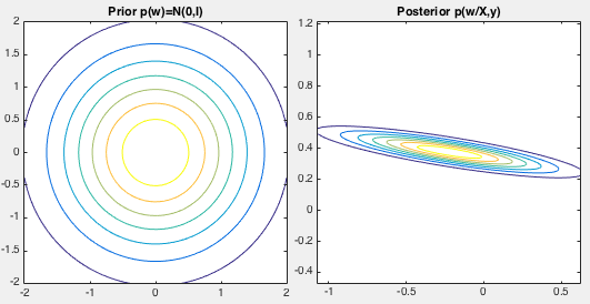
where we have assumed $x_0=1$, $w_0=-1/2$ and $w_1=1/2$, i.e., the function is actually a straight line $f(x)=(-1+x)/2$ with intercept $w_0=-1/2$ and slope $w_1=1/2$. The distribution of the additive noise (residual) is $p(e)={\cal N}(0,\,\sigma_r=0.8)$. The prior distributions of the weights ${\bf w}=[w_0,w_1]^T$ is assumed to be $p({\bf w})={\cal N}({\bf0},{\bf I})$, and posterior $p({\bf w}\vert{\cal D})$ can be obtained based on the observed data ${\cal D}=\{ {\bf X},{\bf y}\}$, both shown in the figure below. We see that the posterior is concentrated around $\hat{w}_1=-0.28$ and $\hat{w}_2=0.39$, the estimates of the true weights $w_1=-0.5$ and $w_2=0.5$, based on the observed noisy data.

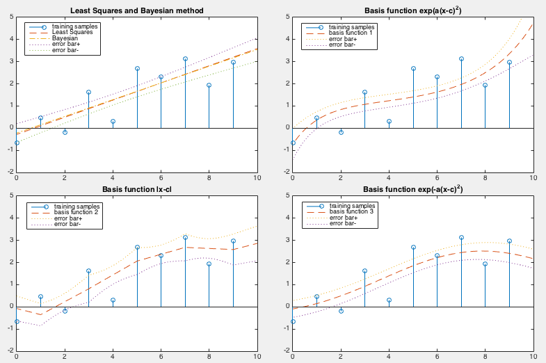
Various regression methods including both the least-squared method and the Bayesian linear regression methods, and in feature space spanned by a set of basis functions $\phi_i({\bf x}),\;(i=1,\cdots,D=5)$ based on each of the three functions given above are carried out with their results shown in the figure below:

The LS errors for these methods are listed below:

$$\begin{array}{c\vert\vert c\vert c}\hline \mbox{Method} & \mb... ...rt{\bf x}-{\bf c}\vert\vert^2) & 0.4459 & \\ \hline \end{array}$$ (186)

We see that the linear methods (the pseudo inverse and the Bayesian regression) produce similar estimated weights error, but smaller error can be achieved by the same method of Bayesian linear regression if proper nonlinear mapping is used (e.g., the last two mapping functions).