Linear Least Squares Regression

In linear regression, the relationship between the dependent variable $y$ and $d$ independent variables in ${\bf x}=[x_1,\cdots,x_d]^T$ is modeled by a linear hypothesis function:

$$\hat{y}=f({\bf x},{\bf w})=b+\sum_{i=1}^d w_ix_i =\sum_{i=0}^d w_ix_i={\bf x}^T{\bf w}$$ (108)

where ${\bf x}=[x_0=1,x_1,\cdots,x_d]^T$ is redefined as an augmented $d+1$ dimensional vector containing $x_0=1$ as well as the $d$ independent variables, and ${\bf w}=[w_0=b,w_1,\cdots,w_d]^T$ is an argmented $d+1$ dimensional vector containing $w_0=b$ as well as the $d$ weights as the parameters, to be determined based on the given dataset.

Geometrically, this linear regression function $f({\bf x})={\bf w}^T{\bf x}$ is a straight line if $d=1$, a plane if $d=2$, or a hyperplane if $d>2$, in the $d+1$ dimensional space spanned by $y$ as well as $\{x_1,\cdots,x_d\}$. The function has an intercept $f({\bf0})=w_0=b$ along the $y$ dimension and a normal direction $[w_1,\cdots,w_d,\,-1]^T$. When thresholded by the plane $y=0$, the regression function becomes an equation $f({\bf x})={\bf x}^T{\bf w}=0$, representing a point if $d=1$, a straight line if $d=2$, a plane or hyperplane if $d\ge 3$, in the d-dimensional space spanned by $\{x_1,\cdots,x_d\}$, as shown in the figure below for $d=2$.

We denote by ${\bf X}$ the matrix containing the $N$ augmented data points ${\bf x}_n=[x_{0n}=1,\,x_{1n},\cdots,x_{dn}]^T\;(n=1,\cdots,N)$ as its column vectors

$${\bf X}=\left[\begin{array}{ccc}1 &\cdots&1\\ x_{11}&\cdots&x_{1N... ...}&\cdots&x_{dN}\end{array}\right]_{(d+1)\times N} =[{\bf x}_1,\cdots,{\bf x}_N]$$ (109)

and its transpose can be written as:

$${\bf X}^T=\left[\begin{array}{cccc}1 & x_{11} & \cdots & x_{d1} \... ...imes(d+1)} =\left[{\bf 1},\underline{\bf x}_1,\cdots,\underline{\bf x}_d\right]$$ (110)

where ${\bf 1}=[1,\cdots,1]^T$, and $\underline{\bf x}_i=[x_{i1},\cdots,x_{iN}]^T\;\;(i=1,\cdots,d)$ is an N-dimensional vectors containing the ith components of all $N$ data vectors in the dataset.

Now the linear regression problem is simply to find the model parameter, here the weight vector ${\bf w}$, so that the model prediction

$$\hat{\bf y}={\bf X}^T{\bf w}$$ (111)

matches the ground truth labeling ${\bf y}$. In other words, the residual of the linear model defined as ${\bf r}={\bf y}-{\bf X}^T{\bf w}$ need to be zero:

$${\bf r}={\bf y}-{\bf X}^T{\bf w}={\bf0}$$ (112)

This is a linear system containing $N$ equations of $M$ unknowns.

If the number of data samples is equal to the number of unknown parameters, i.e., $N=d+1$, then ${\bf X}$ is a square and invertible matrix (assuming all $N$ samples are independent and therefore ${\bf X}$ has a full rank), and the equation above can be solved to get the desired weight vector:

$${\bf w}=({\bf X}^T)^{-1}{\bf y}$$ (113)

However, as typically $N \gg d+1$, i.e., there are many more data samples than the unknown parameters, ${\bf X}$ is non-invertible and ${\bf X}^T{\bf w}={\bf y}$ is over-determined linear system without a solution, i.e, the prediction $\hat{y}={\bf X}^T{\bf w}$ can never match the ground truth labeling ${\bf y}$. We need to find an optimal solution ${\bf w}^*$ that minimizes the SSE (proportional to MSE):

$$\varepsilon({\bf w}) = \frac{1}{2}\sum_{n=1}^B r_n^2 =\frac{1}{2}\vert\vert{\bf r}\vert\vert^2 =\frac{1}{2}\vert\vert{\bf y}-{\bf X}^T{\bf w}\vert\vert^2$$

$$= \frac{1}{2}{\bf y}^T{\bf y}-{\bf y}^T{\bf X}^T{\bf w} +\frac{1}{2}{\bf w}^T{\bf X}{\bf X}^T{\bf w}$$ (114)

To find the optimal ${\bf w}$ that minimizes $\varepsilon({\bf w})$, we set the gradient of $\varepsilon$ to zero and get the normal equation:

$${\bf g}_\varepsilon({\bf w})=\frac{d}{d{\bf w}} \varepsilon({\bf w}) ={\bf XX}^T{\bf w}-{\bf Xy}={\bf0}, \;\;\;\;\; \;\;\;\;\; {\bf XX}^T{\bf w}={\bf Xy}$$ (115)

Solving for ${\bf w}$, we get the optimal weight vector:

$${\bf w}^*=({\bf X}{\bf X}^T)^{-1}{\bf X}{\bf y}=({\bf X}^T)^-{\bf y}$$ (116)

where $({\bf X}^T)^-=({\bf X}{\bf X}^T)^{-1}{\bf X}$ is the $(d+1)\times N$ pseudo-inverse of the $N\times(d+1)$ matrix ${\bf X}^T$. This method for estimating the regression model parameters is called ordinary least squares (OLS).

Having found the parameter ${\bf w}$ for the linear regression model $\hat{y}={\bf x}^T{\bf w}$, we can predict the outputs corresponding to any unlabed test dataset ${\bf X}_*=[{\bf x}_{1*},\cdots,{\bf x}_{M*}]$:

$$\hat{\bf y}_*={\bf f}_*={\bf X}_*^T{\bf w}^* =[{\bf 1},\underline... ...s\\ w^*_d\end{array}\right] =w^*_0{\bf 1}+\sum_{i=1}^d w^*_i\underline{\bf x}_i$$ (117)

which is a linear combination of ${\bf 1}$ and $\{\underline{\bf x}_1,\cdots,\underline{\bf x}_d\}$

We further consider the evaluation of the linear regression result in terms of how well it fits the training data. We first rewrite the normal equation in Eq. (115) as:

$${\bf XX}^T{\bf w}-{\bf Xy}={\bf X} \left( {\bf X}^T{\bf w}-{\bf y}\right) ={\bf X}\left( \hat{\bf y}-{\bf y}\right)$$

$$= {\bf Xr}=\left[\begin{array}{ccc}1 & \cdots & 1\\ x_{11}&\cdots&x... ...ne{\bf x}_1^T\\ \vdots\\ \underline{\bf x}_d^T \end{array}\right]{\bf r}={\bf0}$$ (118)

The last equality indicate that the residual vector ${\bf r}$ is parpendicular to each of the $d+1$ vectors $\{ {\bf 1},\underline{\bf x}_1,\cdots,\underline{\bf x}_d\}$:

$${\bf 1}^T{\bf r}=\sum_{n=1}^Nr_n=0,\;\;\;\;\; \underline{\bf x}_1^T{\bf r}=\cdots=\underline{\bf x}_N^T{\bf r}=0$$ (119)

We see that the residual ${\bf r}={\bf y}-\hat{\bf y}={\bf y}-{\bf X}^T{\bf w}^*$ based on the optimal ${\bf w}^*$ represents the shortest distance between ${\bf y}$ and any point in the space spanned by $\{ {\bf 1},\underline{\bf x}_1,\cdots,\underline{\bf x}_d\}$, i.e., any other estimate $\hat{\bf y}'={\bf X}^T{\bf w}$ also in the space but based on a non-optmal ${\bf w}\ne{\bf w}^*$ must have a greater residual ${\bf r}'={\bf y}-\hat{\bf y}'\;>\;{\bf r}$, i.e., ${\bf w}^*$ is indeed the optimal parameter based on which the sum of quared error $\vert\vert{\bf r}\vert\vert^2$ of the model $\hat{\bf y}={\bf X}^T{\bf w}^*$ is minimized.

We further consider some quantitative measurement for evaluating how well the linear regression model $y={\bf w}^T{\bf x}$ fits the given dataset. To do so, we first derive some properties of the model based on its output $\hat{\bf y}={\bf X}^T{\bf w}={\bf X}^T({\bf XX}^T)^{-1}{\bf Xy}$:

$$\vert\vert\hat{\bf y}\vert\vert^2 = \hat{\bf y}^T\hat{\bf y} =\left({\bf X}^T({\bf XX}^T)^{-1}{\bf Xy}\right)^T \; \left({\bf X}^T({\bf XX}^T)^{-1}{\bf Xy}\right)$$

$$= \left({\bf y}^T{\bf X}^T ({\bf XX}^T)^{-1}{\bf X}\right)\; \left({\bf X}^T({\bf XX}^T)^{-1}{\bf Xy}\right)$$

$$= {\bf y}^T{\bf X}^T ({\bf XX}^T)^{-1}{\bf Xy}={\bf y}^T\hat{\bf y}$$ (120)

based on which we also get

$${\bf r}^T\hat{\bf y}=({\bf y}-\hat{\bf y})^T\hat{\bf y} ={\bf y}^T\hat{\bf y}-\hat{\bf y}^T\hat{\bf y}=0$$ (121)

$$\vert\vert{\bf r}\vert\vert^2 = {\bf r}^T{\bf r} =({\bf y}-\hat{\bf y})^T\;({\bf y}-\hat{\bf y}) ={\bf y}^T{\bf y}-2{\bf y}^T\hat{\bf y}+\hat{\bf y}^T\hat{\bf y}$$

$$= {\bf y}^T{\bf y}-{\bf y}^T\hat{\bf y} ={\bf y}^T({\bf y}-\hat{\bf y}) ={\bf y}^T{\bf r}$$ (122)

and

$$\vert\vert\hat{\bf y}\vert\vert^2+\vert\vert{\bf r}\vert\vert^2={... ...{\bf y}^T( \hat{\bf y}+{\bf r} )={\bf y}^T{\bf y}=\vert\vert{\bf y}\vert\vert^2$$ (123)

We further find the mean of $\{y_1,\cdots,y_N\}$

$$\bar{y}=\frac{1}{N}\sum_{n=1}^N y_n=\frac{1}{N}{\bf y}^T{\bf 1}$$ (124)

and define a vector $\bar{\bf y}=\bar{y}\;{\bf 1}$. The three vectors ${\bf y}-\hat{\bf y}$, ${\bf y}-\bar{\bf y}$ and $\hat{\bf y}-\bar{\bf y}$ are all perpendicular to vector ${\bf 1}$:

$$({\bf y}-\bar{\bf y})^T{\bf 1} = \sum_{n=1}^N(y_n-\bar{y}) =N(\bar{y}-\bar{y})=0$$

$$({\bf y}-\hat{\bf y})^T{\bf 1} = \sum_{n=1}^N(y_n-\hat{y}_n) =\sum_{n=1}^N r_n=0\;\;\;\;\;\;\;Eq. (\ref{sumofrzero})$$

$$(\hat{\bf y}-\bar{\bf y})^T{\bf 1} = (\hat{\bf y}-{\bf y}+{\bf y}-\bar{\bf y})^T{\bf 1} =(\hat{\bf y}-{\bf y})^T{\bf 1}+({\bf y}-\bar{\bf y})^T{\bf 1} =0$$ (125)

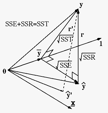
Based on these three vectors, we further define the following sums of squares:

• The total sum of squares (TSS) for the total variation in data:

  $$TSS=\vert\vert{\bf y}-\bar{\bf y}\vert\vert^2=\sum_{n=1}^N(y_n-\bar{y})^2$$ (126)

• The explained sum of squares (ESS) for the variation of data explained by the regression model:

  $$ESS=\vert\vert\hat{\bf y}-\bar{\bf y}\vert\vert^2=\sum_{n=1}^N (\hat{y}_n-\bar{y})^2$$ (127)

• Residual sum of squares (RSS) for the variation of data not explained by the data (due to noise or discrepancy between the data and the model):

  $$RSS=\vert\vert{\bf r}\vert\vert^2=\vert\vert{\bf y}-\hat{\bf y}\vert\vert^2=\sum_{n=1}^N (y_n-\hat{y}_n)^2$$ (128)

We can show that the total sum of squares is the sum of the explained sum of squares and the residual sum of squares:

$$TSS = \vert\vert{\bf y}-\bar{\bf y}\vert\vert^2 =\vert\vert{\bf y}-\bar... ...t\vert^2 =\vert\vert(\hat{\bf y}-\bar{\bf y})+({\bf y}-\hat{\bf y})\vert\vert^2$$

$$= \vert\vert\hat{\bf y}-\bar{\bf y}\vert\vert^2 +2({\bf y}-\hat{\bf y})^T(\hat{\bf y}-\bar{\bf y}) +\vert\vert{\bf y}-\hat{\bf y}\vert\vert^2$$

$$= \vert\vert\hat{\bf y}-\bar{\bf y}\vert\vert^2+2{\bf r}^T(\hat{\bf y}-\bar{\bf y})+\vert\vert{\bf r}\vert\vert^2$$

$$= ESS+2{\bf r}^T\hat{\bf y}-2{\bf r}^T\bar{\bf y}+RSS =ESS+RSS$$ (129)

The last equality is due to the fact that the two middle terms are both zero:

$$\left\{ \begin{array}{l} {\bf r}^T\... ...bf y}-\hat{\bf y}^T\hat{\bf y}=0\;\;\; Eq. (\ref{y2eqyyh} ) \end{array} \right.$$ (130)

We can now measure the goodness of the model by the coefficient of determination, denoted by $R^2$ (R-squared), defined as the percentage of variance explained by the model:

$$R^2=\frac{ESS}{TSS}=1-\frac{RSS}{TSS}$$ (131)

Given the total sum of squares TSS, if the model residual RSS is small, then ESS is large, indicating most of the variation in the data can be explained by the model, and $R^2$ is large, i.e., the model is a good fit of the data.

In the special case of 1-dimensional dataset $\{(x_n,\,y_n)\;\;(n=1,\cdots,N)\}$, how closely the two variables $x$ and $y$ are correlated to each other can be measured by correlation coefficient defined as:

$$\rho=\frac{\sigma_{xy}^2}{\sqrt{\sigma_x^2\;\sigma_y^2}} =\frac{\sigma_{xy}^2}{\sigma_x\;\sigma_y}$$ (132)

where

$$\bar{x}=\frac{1}{N}\sum_{n=1}^Nx_n,\;\;\;\;\bar{y}=\frac{1}{N}\sum_{n=1}^Ny_n$$

and

$$\sigma_x^2=\frac{1}{N}\sum_{n=1}^N x_n^2-\bar{x}^2,\;\;\;\;\; \si... ...r{y}^2,\;\;\;\;\;\; \sigma_{xy}^2=\frac{1}{N}\sum_{n=1}^N x_ny_n-\bar{x}\bar{y}$$

A few simple examples of different correlation coefficients can be found here.

We can further find the linear regression model $y=w_0+w_1\,x$ in terms of the model parameters:

$${\bf w} = \left[\begin{array}{c}w_0\\ w_1\end{array}\right] =({\bf X}{\bf X... ..._N\end{array}\right] \left[\begin{array}{c}y_1\\ \vdots\\ y_N\end{array}\right]$$

$$= \left[\begin{array}{ccc}N&\sum_{n=1}^Nx_n\\ \sum_{n=1}^Nx_n&\sum_... ...\left[\begin{array}{c}\bar{y}\\ \sigma_{xy}^2+\bar{x}\bar{y} \end{array}\right]$$

$$= \frac{1}{\sigma_x^2} \left[\begin{array}{ccc}\sigma_x^2+\bar{x}^2... ...sigma_{xy}^2/\sigma_x^2 \;\bar{x}\\ \sigma_{xy}^2/\sigma_x^2\end{array}\right]$$ (133)

Based on these model parameters $w_1=\sigma_{xy}^2/\sigma_x^2$ and $w_0=\bar{y}-\bar{x} w_1$, we get the linear regression model:

$$\hat{y}=w_0+w_1 x =\bar{y}-\frac{\sigma_{xy}^2}{\sigma_x^2}\bar{x}+\frac{\sigma_{xy}^2}{\sigma_x^2}x \;\;\;\;\;\; \;\;\;\;\;\;\; \frac{\sigma_{xy}^2}{\sigma_x^2}=\frac{y-\bar{y}}{x-\bar{x}}$$ (134)

The coefficient of determination $R^2$ for the goodness of the regression is closely related to the correlation coefficient $\rho$ for correlation of the given data (but independent of the model), as one would intuitively expect. Consider

$$\frac{1}{N}RSS = \frac{1}{N}\vert\vert y-\hat{y}\vert\vert^2 =\frac{1}{N}\sum_{n=1}^N(y_n-w_0-w_1x_n)^2 =\frac{1}{N}\sum_{n=1}^N(y_n-(\bar{y}-\bar{x} w_1)-w_1x_n)^2$$

$$= \frac{1}{N}\sum_{n=1}^N[(y_n-\bar{y})-w_1(x_n-\bar{x})]^2 =\frac{... ...um_{n=1}^N[(y_n-\bar{y})^2-2w_1(y_n-\bar{y})(x_n-\bar{x})+w_1^2(x_n-\bar{x})^2]$$

$$= \sigma_y^2-2w_1\sigma^2_{xy}+w_1^2 \sigma_x^2 =\sigma_y^2-2\frac{... ...igma^4_{xy}}{\sigma^4_x}\sigma_x^2 =\sigma_y^2-\frac{\sigma^4_{xy}}{\sigma^2_x}$$

$$= \sigma_y^2\left(1-\frac{\sigma^4_{xy}}{\sigma_x^2\sigma_y^2}\right) =\sigma_y^2(1-\rho^2)$$ (135)

We see that if the two variables $x$ and $y$ are highly correlated and $\rho$ is close to 1, then the error of the model is small, i.e., $RSS=\vert\vert{\bf r}\vert\vert^2$ is small and $R^2$ is large, indicating the LS linear model fits the data well.

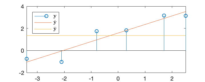
Example 1:

Find a linear regression function $y=w_0+w_1\,x$ to fit the following $N=6$ points:

$$\begin{tabular}{r\vert\vert r\vert r\vert r\vert r\vert r\vert r}... ... \hline y & -0.76 & -1.04 & 1.75 & 1.82 & 3.17 & 3.15\\ \hline \end{tabular}\\$$

Based on the data, we get

$$\bar{y}=1.348,\;\;\;\sigma^2_x=4.22,\;\;\;\sigma^2_y=2.85,\;\;\; \sigma^2_{xy}=3.27,\;\;\;\; \rho=\frac{\sigma^2_{xy}}{\sigma_x\sigma_y}=0.94 \\$$

The augmented data array is:

$${\bf X}=\left[\begin{array}{cccccc}1&1&1&1&1&1\\ -3.4 & -2.1 & -0.8 & 0.3 & 1.7 & 2.5 \end{array}\right] \\$$

Solving the over-constrained equation system

$${\bf y}=\left[\begin{array}{c}-0.76\\ -1.04\\ 1.75\\ 1.82\\ 3.17\... ... 1&2.5 \end{array}\right] \left[\begin{array}{c}w_0\\ w_1\end{array}\right] \\$$

we get

$${\bf w}={\bf X}^- {\bf y}=({\bf X}{\bf X}^T)^{-1}{\bf X}\;{\bf y}... ....15 \end{array}\right] =\left[\begin{array}{c}1.58\\ 0.78\end{array}\right] \\$$

and the linear regression model function $y=w_0+w_1\,x=1.58+0.78\,x$, a straight line with intercept $w_0=1.58$, slope $w_1=0.78$, and normal direction $[0.78,\;-1]^T$. The LS error is $\vert\vert{\bf r}\vert\vert=\vert\vert{\bf y}-\hat{\bf y}\vert\vert=1.38$. We can further get $\bar{\bf y}=[1.348,\;1.348,\;1.348,\;1.348,\;1.348,\;1.348]^T$, $\hat{\bf y}={\bf X}^T{\bf w}=[-1.054,\;-0.047,\;0.961,\;1.813,\;2.898,\;3.518]^T$, and

$$ESS=15.21,\;\;RSS=1.91,\;\;TSS=17.12,\;\;R^2=0.89$$

We can also check that

$$\frac{1}{N} RSS = \sigma_y^2(1-\rho^2)=0.318$$

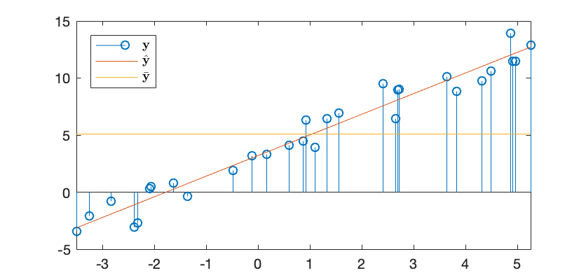
Example 2:

$$\begin{tabular}{c\vert\vert c\vert c\vert c\vert c\vert c\vert c\... ... -7.29 & 8.31 & 0.98 & 10.18 & 8.58 &10.86 & 0.77 & 0.20\\ \hline \end{tabular}$$

$$\begin{tabular}{c\vert\vert c\vert c\vert c\vert c\vert c\vert c\... ... 0.91 & 1.92 & 166.98 & 443.92 & 610.89 & 0.273 & 0.523 \\ \hline \end{tabular}$$

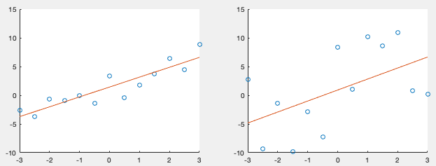
Example 3:

The figure below shows a set of $N=30$ data points $\{(x_i,\,y_i),\;i=1,\cdots,30\}$ fitted by a 1-D linear regression function $y=w_0+w_1 x$, a straight line, with $w_0=1.81,\;w_1=3.22$. The correlation coefficient is $\rho=0.98$, and $ESS=734.78,\;\;RSS=32.98,\;\;TSS=767.77$, $R^2=0.96$.

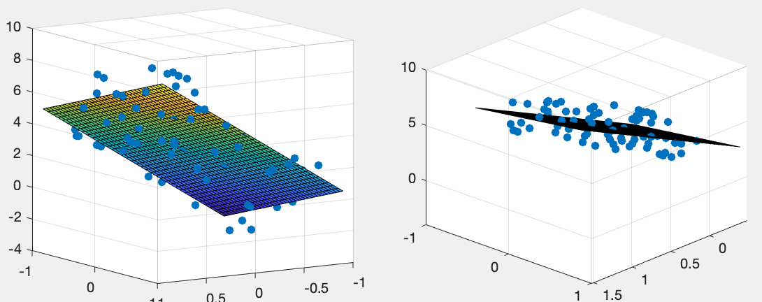
Example 4:

The figure below shows a set of $N=90$ data points $\{({\bf x}_i,\,y_i),\;i=1,\cdots,90\}$ fitted by a 2-D linear regression function $y=w_0+w_1x_1+w_2x_2$, a plane, with $w_0=2.82,\;w_1=1.85,\;w_2=4.31$„ and $ESS=677.00, RSS=124.48,\;TSS=802.47$ and $R^2=0.84$.