Next: Gradient Descent Method Up: Unconstrained Optimization Previous: Nelder-Mead method
Newton's method is based on the
Taylor series expansion
of the function  to be minimized near some point
  :
:
 |
 |
 |
|
 |
 |
(28) |
If  is a quadratic function, then the Taylor series
contains only the first three terms (constant, linear, and quadratic
terms). In this case, we can find the vertex point at which
is a quadratic function, then the Taylor series
contains only the first three terms (constant, linear, and quadratic
terms). In this case, we can find the vertex point at which  reaches its extremum, by first setting its derivative to zero:
 |
|
![$\displaystyle \frac{d}{dx}q(x)=\frac{d}{dx}\left[ f(x_0)+f'(x_0)(x-x_0)
+\frac{1}{2}f''(x_0)(x-x_0)^2 \right]$](img161.svg) |
|
|
 |
(29) |
 to get:
where
to get:
where
 is the step we need to take
to go from any initial point to the solution
is the step we need to take
to go from any initial point to the solution  in a
single step. Note that
in a
single step. Note that  is a minimum if
 but
a maximum if
but
a maximum if
 .
.
If
 is not quadratic, the result above can still
be considered as an approximation of the solution, which can be
improved iteratively from the initial guess to eventually
approach the solution:
is not quadratic, the result above can still
be considered as an approximation of the solution, which can be
improved iteratively from the initial guess to eventually
approach the solution:
 |
(31) |
 .
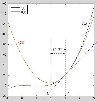
We see that in each step
.
We see that in each step  of the iteration, the function
is fitted by a quadratic functions
of the iteration, the function
is fitted by a quadratic functions  and its vertex
at
and its vertex
at  is used as the updated approximated solution, at
which the function is again fitted by another quadratic function
is used as the updated approximated solution, at
which the function is again fitted by another quadratic function
 for the next iteration. Through this process the
solution can be approached as
for the next iteration. Through this process the
solution can be approached as
 .
.
We note that the iteration
 is just
the Newton-Raphson method
for equation
is just
the Newton-Raphson method
for equation  , as a necessary condition for an extremum
of .
, as a necessary condition for an extremum
of .
Newton's method for the minimization of a single-variable
function can be generalized for the minimization of
a mult-variable function
 . Again,
we approximate
. Again,
we approximate
 by a quadratic function
 containing only the first three terms of its
Taylor series
at some initial point
containing only the first three terms of its
Taylor series
at some initial point  :
:
 |
(32) |
 and
and  are respectively the gradient vector and
Hessian matrix of the function
at :
are respectively the gradient vector and
Hessian matrix of the function
at :
 |
|
![$\displaystyle {\bf g}_f({\bf x}_0)=\frac{d}{d{\bf x}} f({\bf x}_0)
=\left[\begi...
...x_1}\\
\vdots \\ \frac{\partial f({\bf x}_0)}{\partial x_N}\end{array}\right],$](img185.svg) |
|
 |
|
![$\displaystyle {\bf H}_f({\bf x}_0)=\frac{d}{d{\bf x}} {\bf g}({\bf x}_0)
=\frac...
...1} &
\cdots & \frac{\partial^2 f({\bf x}_0)}{\partial x_N^2}
\end{array}\right]$](img187.svg) |
(33) |
 can be found
from any point by setting its derivative to zero
can be found
from any point by setting its derivative to zero
 |
|
![$\displaystyle \frac{d}{d{\bf x}}\left[f({\bf x}_0)+{\bf g}_0^T({\bf x}-{\bf x}_0)
+\frac{1}{2}({\bf x}-{\bf x}_0)^T{\bf H}_0\,({\bf x}-{\bf x}_0)\right]$](img190.svg) |
|
|
 |
(34) |
 |
(35) |
 is either a
minimum or maximum depends on whether the second order derivative
is either a
minimum or maximum depends on whether the second order derivative
 is greater or smaller than zero, here whether
is a minimum, maximum, or neither, depends on the
second order derivatives, the Hessiam matrix
is greater or smaller than zero, here whether
is a minimum, maximum, or neither, depends on the
second order derivatives, the Hessiam matrix
 :
:
 is positive definite (all eigenvalues are positive),
is a local minimum;
is positive definite (all eigenvalues are positive),
is a local minimum;
 is negative definite (all eigenvalues are negative),
a local maximum;
is negative definite (all eigenvalues are negative),
a local maximum;
 is indefinite (has both positive and negative
eigenvalues),
is a saddle point (neither minimum nor
maximum).
is indefinite (has both positive and negative
eigenvalues),
is a saddle point (neither minimum nor
maximum).
If
 is not quadratic, the result above is
not a minimum or maximum, but it can still be used as an approximation
of the solution, which can be improved to approached the true solution
iteratively:
is not quadratic, the result above is
not a minimum or maximum, but it can still be used as an approximation
of the solution, which can be improved to approached the true solution
iteratively:
 ,
,
 ,
and the increment
,
and the increment
 is called Newton search direction. We note that the
computational complexity for each iteration is
is called Newton search direction. We note that the
computational complexity for each iteration is  due to the
inverse operation
due to the
inverse operation
 .
.
We note that the iteration above is just a generalization of
in 1-D case where
 and
and
 . Also, the iteration
 above is just the
Newton-Raphson method
for
solving equation
above is just the
Newton-Raphson method
for
solving equation
 as the necessary condition for an extremum of
 .
.
The speed of convergence of the iteration can be controlled by a
parameter  that controls the step size:
 |
(37) |
Example:
An over-constrained nonlinear equation system
 of
of  equations and
  unknowns can be solved by minimizing the following
sum-of-squares error:
unknowns can be solved by minimizing the following
sum-of-squares error:
 |
(38) |
The gradient of the error function is:
 |
(39) |
 |
(40) |
 is the component
of the function's Jacobian
is the component
of the function's Jacobian
 in the mth
row and ith column.
in the mth
row and ith column.
We further find the component of the Hessian
 of the error function in the ith row and jth column:
 |
|
![$\displaystyle \frac{\partial^2}{\partial x_i\partial x_j}\frac{1}{2}\vert\vert{...
...frac{\partial}{\partial x_j}
\left[ f_m\frac{\partial f_m}{\partial x_i}\right]$](img217.svg) |
|
|
![$\displaystyle \sum_{m=1}^M \left[
\frac{\partial f_m}{\partial x_i}\;\frac{\par...
...f_m}{\partial x_j}
+f_m \frac{\partial^2 f_m}{\partial x_i\partial x_j} \right]$](img218.svg) |
||
|
 |
(41) |
 .
Now the Hessian can be written as
.
Now the Hessian can be written as
 |
(42) |
 that minimizes
 can be found iteratively:
 |
(43) |
![[*]](crossref.png) ) in the
previous chapter.
) in the
previous chapter.
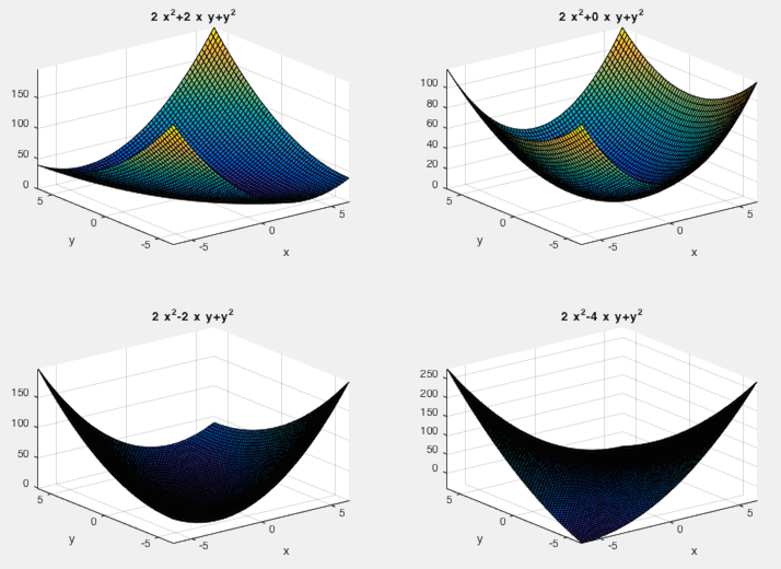
Example:
Consider the following quadratic function:
![$\displaystyle q(x,y)=\frac{1}{2} [x_1,\;x_2]
\left[\begin{array}{cc}a&b/2\\ b/2...
...\begin{array}{c}x_1\\ x_2\end{array}\right]
=\frac{1}{2}(ax_1^2+bx_1x_2+cx_2^2)$](img224.svg) |
![$\displaystyle {\bf g}=\left[\begin{array}{c}ax_1+bx_2/2\\ bx_1/2+cx_2\end{array...
...gin{array}{cc}a&b/2\\ b/2&c\end{array}\right],
\;\;\;\;\;\;\det{\bf H}=ac-b^2/4$](img225.svg) |
 ,
,  , and consider the following values of
  :
:
 ,
,
 ,
,
 ,
,
 ,
,
 is positive definite,
 is the minimum.
 ,
,
 ,
,
 ,
,
 ,
is positive definite,
is the minimum.
,
is positive definite,
is the minimum.
 ,
,
,
,
is positive definite,
is the minimum.
,
,
,
,
is positive definite,
is the minimum.
 ,
,
 ,
,
 ,
,
 ,
,
 is indefinite,
is a saddle point (minimum in one direction
but maximum in another).
is indefinite,
is a saddle point (minimum in one direction
but maximum in another).
We can speed up the convergence by a bigger step size  . However,
if
. However,
if  is too big, the solution may be skipped and the iteration may
not converge if it gets into an oscillation around the solution. Even worse,
the iteration may become divergent. For such reasons, a smaller step size
is too big, the solution may be skipped and the iteration may
not converge if it gets into an oscillation around the solution. Even worse,
the iteration may become divergent. For such reasons, a smaller step size
 may be preferred sometimes.
In summary, Newton's method approximates the function
at an
estimated solution  by a quadratic equation (the first three
terms of the Taylor's series) based on the gradient
by a quadratic equation (the first three
terms of the Taylor's series) based on the gradient  and Hessian
of the function at , and treat the vertex of the
quadratic equation as the updated estimate
and Hessian
of the function at , and treat the vertex of the
quadratic equation as the updated estimate
 .
.
Newton's method requires the Hessian matrix as well as the gradient to be available. Moreover, it is necessary calculate the inverse of the Hessian matrix in each iteration, which may be computationally expensive.
Example:
The Newton's method is applied to solving the following non-linear equation
system of  variables:
 |
 . These equations can
be expressed in vector form as
and solved as an
optimization problem with the objective function
. These equations can
be expressed in vector form as
and solved as an
optimization problem with the objective function
 . The iteration from an
initial guess
. The iteration from an
initial guess
 is shown below.
 |
(44) |
 :
:
![$\displaystyle {\bf x}^*=\left[\begin{array}{r}0.5000008539707297\\ 0.0032017070323056\\
-0.4999200212218281\end{array}\right]$](img257.svg) |
(45) |

