Next: Softmax Regression for Multiclass Up: Regression Analysis and Classification Previous: Nonlinear Least Squares Regression
All previously discussed regression methods can be considered
as supervised binary classifiers, when the regression function
 is thresholded by some constant
  .
Without loss of generality, we will always assume
.
Without loss of generality, we will always assume  in the
following. Once the model parameter
in the
following. Once the model parameter
 is obtained
based on the training set
is obtained
based on the training set
 , every
point
, every
point  in the d-dimensional feature space can be
classified into either of two classes
in the d-dimensional feature space can be
classified into either of two classes  and
and  :
:
if then then |
(207) |
, it
becomes an equation
 representing a hypersurface
in the d-dimensional space (a point if
representing a hypersurface
in the d-dimensional space (a point if  , a curve if
  ,
a surface or hypersurfaceif
,
a surface or hypersurfaceif  ), by which the space is
partitioned into two regions. In this case,
), by which the space is
partitioned into two regions. In this case,
 is
called the decision function and the surface
decision boundary. Now any point in the space is classified
into either of the two classes, depending on whether it is on the
positive side of the decision boundary (
is
called the decision function and the surface
decision boundary. Now any point in the space is classified
into either of the two classes, depending on whether it is on the
positive side of the decision boundary (
 ) or the
negative side (
) or the
negative side (
 ).
).
This simple binary classifier suffers from the drawback that
the distance between a point and the decision boundary
is not taken into consideration, as all points
on the same side of the boundary, regardless how far from the
boundary, are equally classified into the same class. On the
other hand, one would naturally feel more confident about such
a classification for a point far away from the boundary, than a
point very close to it.
This problem can be addressed by the method of
logistic regression, which is similarly trained based
on the training set with each sample  labeled by a
binary value
labeled by a
binary value
 for either of the two classes
and . While the logistic regression is based on the
linear regression function
for either of the two classes
and . While the logistic regression is based on the
linear regression function
 , which
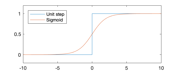
is not hard-thresholded by the unit step function
, which
is not hard-thresholded by the unit step function  to
become either 0 or 1; instead, it is soft-thresholded by a
sigmoid function
to
become either 0 or 1; instead, it is soft-thresholded by a
sigmoid function
 to become a real value between 0 and 1, interpreted as the
probability
to become a real value between 0 and 1, interpreted as the
probability
 for to belong to
, and
for to belong to
, and
 is the
probability for to belong to .
is the
probability for to belong to .
Similar to linear and nonlinear regression methods considered
before, the goal of logistic regression is also to find the
optimal model parameter
for the regression
function
to fit the training set
optimally. But different from linear and nonlinear regression
based on the least squares (LS) method that minimizes the
squared error in Eq. (189), logistic regression is
based on maximum likelihood (ML) estimation,
which maximizes the likelihood of the model parameter,
here
 , as discussed below.
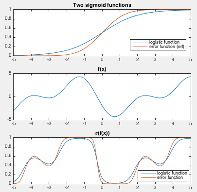
The sigmoid function can be either the error function (cumulative Gaussian, erf):
 |
(208) |
 |
|||
 |
|||
 |
(210) |
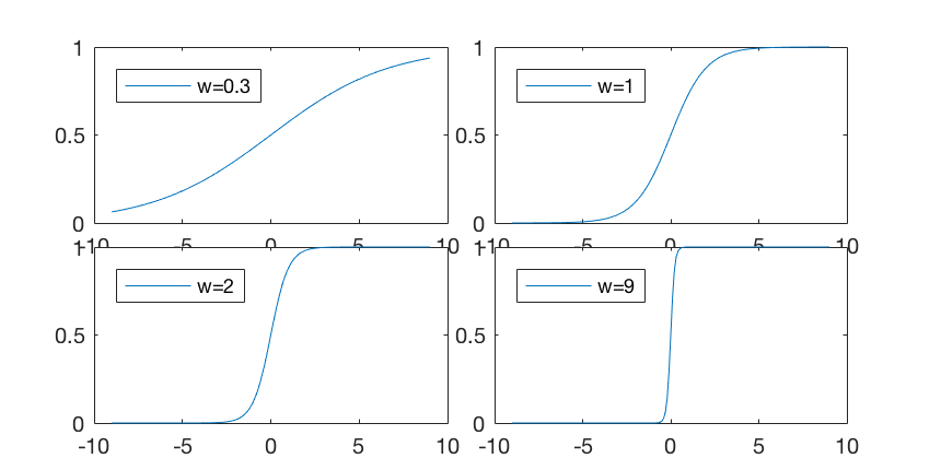
 can be included in the logistic function
to control its softness when used to threshold the variable
can be included in the logistic function
to control its softness when used to threshold the variable  as
shown below:
as
shown below:
 |
(211) |
is thresholded by the logistic
function with variable softness controlled by parameter ,
between the two extreme cases of
 (no
thresholding) when
(no
thresholding) when  , and
, and
 when
when
 (hard thresholding).
Now the function value
 is mapped to
 , treated as the probability
for
, treated as the probability
for
 . Specifically, consider
the following cases:
. Specifically, consider
the following cases:
 , i.e., is
far away from the plane
on the positive side,
then the probability
, i.e., is
far away from the plane
on the positive side,
then the probability
 is close to 1;
 , i.e., is
far away from the plane
on the negative side,
then the probability
is close to 0, but
for
, i.e., is
far away from the plane
on the negative side,
then the probability
is close to 0, but
for
 is close to 1;
 , i.e., is close
to the plane
, then
, i.e., is close
to the plane
, then
 , and
, and
 , i.e.,
the probability for to belong to either or
is about the same.
, i.e.,
the probability for to belong to either or
is about the same.
The value of the logistic function is interpreted as the
conditional probability of output  given data
point and model parameter
given data
point and model parameter  :
:
 is:
is:
 |
(213) |
 (either 1 or 0), as the labeling of a sample
in the training set:
(either 1 or 0), as the labeling of a sample
in the training set:
 |
 |
 |
(214) |
given all
 samples in
(assumed i.i.d.):
samples in
(assumed i.i.d.):
 |
|
 |
|
|
 |
(215) |
can be defined as the
one that maximizes the likelihood function
 ,
or, equivalently, that minimizes the negative log likelihood as
the objective function:
This is the method of maximum likelihood estimation (MLE), and
it produces the most probable estimation of certan parameter
of a model based on the given data.
,
or, equivalently, that minimizes the negative log likelihood as
the objective function:
This is the method of maximum likelihood estimation (MLE), and
it produces the most probable estimation of certan parameter
of a model based on the given data.
The optimal paramter can also be found by the method
of maximum a posteriori (MAP), which maximizes the posterior
probability:
 |
(217) |
 is
the likelihood found above,
is
the likelihood found above,
 is the prior probability
of without observing the training data
is the prior probability
of without observing the training data  , and
the denominator independent of the variable is dropped
as a constant independent of .
, and
the denominator independent of the variable is dropped
as a constant independent of .
Based on the assumption that all components of are
independent of each other and they have zero mean and the same
variance, we let the prior probability be:
 |
(218) |
 is
independent of and is therefore dropped. The
assumed zero mean is due to the desire that the values of
all weights in should be around zero instead
of large values on either positive or negative side, to
avoid overfitting, as discussed below.
is
independent of and is therefore dropped. The
assumed zero mean is due to the desire that the values of
all weights in should be around zero instead
of large values on either positive or negative side, to
avoid overfitting, as discussed below.
Now the posterior can be written as
that maximizes this posterior
 by the mathod
of maximum a posteriori (MAP) estimation. To do so, we
minimize the negative log posterior as the objective function:
by the mathod
of maximum a posteriori (MAP) estimation. To do so, we
minimize the negative log posterior as the objective function:
 as a hyperparameter in
the second term
as a hyperparameter in
the second term
 treated as a penalty
term to discourage large values of , similar to
Eq. (142) for ridge regression. A larger
value of
treated as a penalty
term to discourage large values of , similar to
Eq. (142) for ridge regression. A larger
value of  will result in smaller values for ,
and the logistic function will be more smooth for softer
thresholding, and the classification is less affected by
possible noisy outliers close to the decision boundary. In
other words, by adjusting , we can make a proper
tradeoff between overfitting and underfitting.
will result in smaller values for ,
and the logistic function will be more smooth for softer
thresholding, and the classification is less affected by
possible noisy outliers close to the decision boundary. In
other words, by adjusting , we can make a proper
tradeoff between overfitting and underfitting.
In particular, if
 and
and
 , then
 , i.e., the prior
approaches a uniform distribution (all values of
are equaly likely), then the penalty term can be
removed, and Eq. (220)
becomes the same as Eq. (216),
i.e., the MAP solution that maximizes the posterior
becomes the same as the MLE solution
that maximizes the likelihood
.
, i.e., the prior
approaches a uniform distribution (all values of
are equaly likely), then the penalty term can be
removed, and Eq. (220)
becomes the same as Eq. (216),
i.e., the MAP solution that maximizes the posterior
becomes the same as the MLE solution
that maximizes the likelihood
.
Now we can find the optimal that minimizes
the objective function
 in either
Eq. (216) for the MLE method,
or Eq. (220) for the MAP
method. Here we consider the latter case which is more general
(with an extra term
in either
Eq. (216) for the MLE method,
or Eq. (220) for the MAP
method. Here we consider the latter case which is more general
(with an extra term
 ). We first find
the gradient of objective function:
). We first find
the gradient of objective function:
![$\displaystyle {\bf r}={\bf r}({\bf w})=\left[\begin{array}{c}r_1({\bf w})\\
\v...
...w}^T{\bf x}_1)-y_1\\ \vdots\\
\sigma({\bf w}^T{\bf x}_N)-y_N\end{array}\right]$](img1023.svg) |
(222) |
residuals
 , the difference between the model prediction
 and the ground truth labeling
 . Based on
 we can find the
optimal that minimizes this objective function iteratively
by the gradient descent method.
We note that the gradient in Eq. (221)
is based on all training samples in the training set. If is
large, then the stochastic gradient descent method can be considered
based on only one of the samples in each iteration.
we can find the
optimal that minimizes this objective function iteratively
by the gradient descent method.
We note that the gradient in Eq. (221)
is based on all training samples in the training set. If is
large, then the stochastic gradient descent method can be considered
based on only one of the samples in each iteration.
Below is a segment of Matlab code for estimating by the
gradient descent method. Here X contains the samples
 and
and y contains the corresponding
a binary labelings.
The following code segment estimates weight vector by the
gradient descent method:
    X=[ones(1,n); X];          % augmented X with x_0=1
    w=ones(m+1,1);             % initialize weight vector
    g=X*(sgm(w,X)-y)';         % gradient of log posterior
    tol=10^(-6);               % tolerance
    delta=0.1;                 % step size
    while norm(g)>tol          % terminate when gradient is small enough
        w=w-delta*g;           % update weight vector by gradient descent
        g=X*(sgm(w,X)-y)';     % update gradient
    end
where
    function s=sgm(w,X)
        s=1./(1+exp(-w'*X));
    end
Alternatively, this minimization problem for finding
optimal can also be solved by the
Newton's method
based on the second order
Hessian matrix
 as well as the first order gradient
:
as well as the first order gradient
:
 |
|
 |
|
|
![$\displaystyle {\bf X}\frac{d}{d{\bf w}}\left[\begin{array}{c}
r_1({\bf w})\\ \vdots\\ r_N({\bf w})\end{array}\right]
+\lambda
={\bf X}{\bf J}_r({\bf w})+\lambda$](img1032.svg) |
(223) |
 is the
 Jacobian matrix
of the vector function
Jacobian matrix
of the vector function
 , whose nth row is
![$\displaystyle \frac{dr_n({\bf w})}{d{\bf w}} =\frac{d}{d{\bf w}}
\left[\sigma({...
...\sigma({\bf w}^T{\bf x}_n)[1-\sigma({\bf w}^T{\bf x}_n)]{\bf x}_n
=z_n{\bf x}_n$](img1035.svg) |
(224) |
 ,
which is always greater than zero as
.
Now the Jacobian can be written as
,
which is always greater than zero as
.
Now the Jacobian can be written as
![$\displaystyle {\bf J}_r({\bf w})=\left[\begin{array}{c}dr_1({\bf w})/d{\bf w}\\...
...array}{c}{\bf x}_1^T\\ \vdots\\ {\bf x}_N^T\end{array}\right]
={\bf Z}{\bf X}^T$](img1037.svg) |
(225) |
 is a positive definite diagonal
matrix (as
is a positive definite diagonal
matrix (as  ). Substituting
  back into the expression
for
above, we get
back into the expression
for
above, we get
 |
(226) |
Since  is positive definite, the following quadratic
function is also positive, i.e., for any
is positive definite, the following quadratic
function is also positive, i.e., for any  , we have
 |
(227) |
 is also positive definite, and the objective
function
when approximated by the first three terms of
its Taylor series is has a global minimum.
is also positive definite, and the objective
function
when approximated by the first three terms of
its Taylor series is has a global minimum.
Having found
as well as
 of the objective function
, we can solve the minimization
problem also by the Newton method:
of the objective function
, we can solve the minimization
problem also by the Newton method:
 |
(228) |
by
Newton method:
    X=[ones(1,n); X];          % augmented X with x_0=1
    w=ones(m+1,1);             % initialize weight vector
    g=X*(sgm(w,X)-y)';         % gradient of log posterior
    H=X*diag(s.*(1-s))*X';     % Hesian of log posterior
    tol=10^(-6)
    while norm(g)>tol          % terminate when gradient is small enough
        w=w-inv(H)*g;          % update weight vector by Newton-Raphson
        s=sgm(w,X);            % update sigma
        g=X*(s-y)';            % update gradient
        H=X*diag(s.*(1-s))*X'; % update Hessian
    end
Once the model parameter is available, a given test
sample  of unknown class can be classified into either
of the two classes
of unknown class can be classified into either
of the two classes  and
and  , based on
 :
:
In summary, we make a comparison between the linear and logistic
regression methods both can be used for binary classification. In
linear regression, the function value
is hard-thresholded by the unit step function, so that any data
point is classified to class if
 ,
or class if
,
or class if
 in a deterministic fashion
(with probability
in a deterministic fashion
(with probability
 . On the other
hand, in logistic regression, the linear function
is soft-thresholded by the logistic
function to become
. On the other
hand, in logistic regression, the linear function
is soft-thresholded by the logistic
function to become
 ,
treated as the probability for to belong to class .
Although the same linear model
is
used in both cases, the two methods obtain the model parameter
by minimizing very different objective functions
(Eqs. (114) and
(220)).
,
treated as the probability for to belong to class .
Although the same linear model
is
used in both cases, the two methods obtain the model parameter
by minimizing very different objective functions
(Eqs. (114) and
(220)).


![$\displaystyle J({\bf w})=-l({\bf w}\vert{\cal D})=-\log L({\bf w}\vert{\cal D})...
...g \sigma({\bf w}^T{\bf x}_n)+(1-y_n)\log
(1-\sigma({\bf w}^T{\bf x}_n)) \right]$](img1000.svg)


![$\displaystyle -\sum_{n=1}^N \frac{d}{d{\bf w}}
\left[y_n\log \sigma({\bf w}^T{\bf x}_n)+(1-y_n)\log
(1-\sigma({\bf w}^T{\bf x}_n)) \right]+\lambda{\bf w}$](img1019.svg)

![$\displaystyle \sum_{n=1}^N \left[ \sigma({\bf w}^T{\bf x}_n)-y_n\right]{\bf x}_...
..._1\\ \vdots\\
\sigma({\bf w}^T{\bf x}_N)-y_N\end{array}\right]
+\lambda{\bf w}$](img1021.svg)

 then
then 