Gradient Descent Method

Newton's method discussed above is based on the Hessian ${\bf H}_f({\bf x})$ and gradient ${\bf g}_f({\bf x})$ of the function $f({\bf x})$ to be minimized. However, the method is not applicable if the Hessian ${\bf H}_f$ is not available, or the cost of computing the inverse ${\bf H}^{-1}_f$ is too high. In such a case, the gradient descent method can be used without using the Hessian matrix.

We first consider the minimization of a single-variable function $f(x)$. From any inital point $x_0$, we can move to a nearby point $x_1$ along the opposite direction of the gradient, so that the function value will be smaller than that at the current position $x_0$:

$$x_1=x_0-\delta f'(x_0)=x_0+\Delta x_0 ,\;\;\;\;\; \;\;\;\;\Delta x_0=-\delta f'(x_0),\;\;\;\delta>0$$ (46)

We see that no matter whether $f'(x_0)$ is positive or negative, the function value $f(x_1)$ (approximated by the first two terms of its Taylor series) is always reduced if the positive step size $\delta>0$ is small enough:

$$f(x_1)\approx f(x_0)+f'(x_0)\Delta x_0=f(x_0)-\vert f'(x_0)\vert^2\delta<f(x_0)$$ (47)

This process can be carried out iteratively

$$x_{n+1}=x_n-\delta_n \; f'(x_n),\;\;\;\;\;\;\;n=0,\,1,\,2,\cdots$$ (48)

until eventually reaching a point $x^*$ at which $f'(x^*)=0$ and no further progress can be made, i.e. a local minimum of the function is obtained.

This simple method can be generalized to minimize a multi-variable objective function $f({\bf x})=f(x_1,\cdots,x_N)$ in N-D space. The derivative of the 1-D case is generalized to the gradient vector ${\bf g}({\bf x})=df({\bf x})/d{\bf x}$ of function $f({\bf x})$, which is in the direction along which the function increases most rapidly with the steepest slope, perpendicular to the contour or iso-lines of the function $f({\bf x})$. The fastest way to reduce $f({\bf x})$ is to go down hill along the opposite direction of the gradient vector.

Specifically the gradient descent method (also called steepest descent or down hill method) carries out the following approximation ${\bf x}_{n+1}={\bf x}_n+\Delta{\bf x}_n$ (the first two terms of the Taylor series) with $\Delta{\bf x}=-\delta{\bf g}\;(\delta>0)$:

$$f({\bf x}_1)=f({\bf x}_0+\Delta{\bf x}) \approx f({\bf x}_0)+{\bf... ...T_0 {\bf g}_0 =f({\bf x}_0)-\delta \vert\vert{\bf g}\vert\vert^2 < f({\bf x}_0)$$ (49)

iteratively:

$${\bf x}_{n+1}={\bf x}_n-\delta_n \, {\bf g}_n =({\bf x}_{n-1}-\de... ...{n-1})-\delta_n \, {\bf g}_n=\cdots= {\bf x}_0-\sum_{i=0}^n \delta_n\,{\bf g}_i$$ (50)

untill eventually reaching a point at which ${\bf g}={\bf0}$ and the minimum of the function $f({\bf x})$ is reached.

Comparing the gradient descent method with Newton's method we see that here the Hessian matrix is no longer needed. The iteration simply follows a search direction ${\bf d}_n=-{\bf g}_n$, which is different from the search direction of Newton's method, ${\bf d}_n=-{\bf H}^{-1}_n{\bf g}_n$, based on ${\bf H}_n$ as well as ${\bf g}_n$. Specially, when ${\bf H}={\bf I}$, the two methods become the same.

As the gradient descent method relies only on the gradient vector of the objective function without any information contained in the second order derivatives in the Hessian matrix, it does not have as much information as Newton's method and therefore may not be as efficient. For example, when the function is quadratic, as discussed before, Newton's method can find the solution in a single step from any initial guess, but it may take the gradient descent method many steps to reach the solution, because it always follows the negative direction of the local gradient, which typically does not lead to the solution directly. However, for the same reason, the gradient descent method is computationally less expensive as the Hessian matrix is not used.

Example:

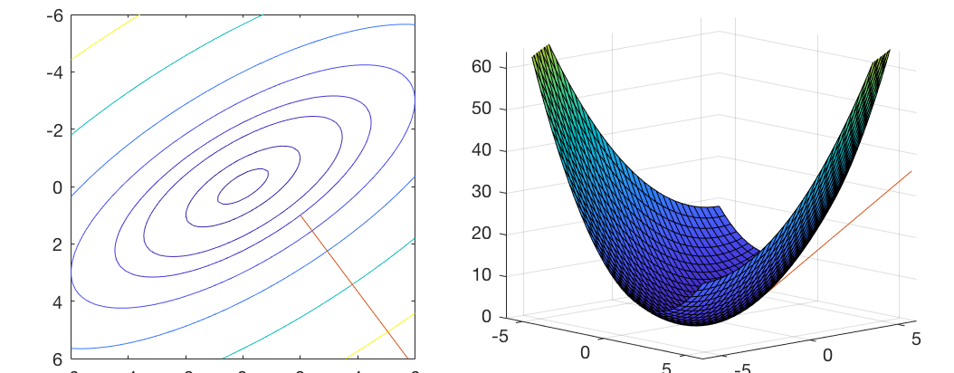
Consider a two-variable quadratic function in the following general form:

$$f({\bf x})={\bf x}^T{\bf Ax}+{\bf b}^T{\bf x}+c =[x_1\;x_2]\left[... ...nd{array}\right] +[b_1\;b_2]\left[\begin{array}{c}x_1\\ x_2\end{array}\right]+c$$

where ${\bf A}$ is a symmetric positive semidefinite matrix, i.e., $a_{12}=a_{21}$ and ${\bf A}\ge 0$. Specially, if we let

$${\bf A}=\left[\begin{array}{cc}2 & 1\\ 1 & 1\end{array}\right],\;\;\;\;\; {\bf b}=\left[\begin{array}{c}0 \\ 0\end{array}\right],\;\;\;\;\; c=0$$

then we have the following function:

$$f(x_1,x_2)=\frac{1}{2}[x_1\;x_2]\left[\begin{array}{cc}2&1\\ 1&1\... ...t[\begin{array}{c}x_1\\ x_2\end{array}\right]=\frac{1}{2}(2x_1^2+2x_1x_2+x_2^2)$$

which has a minimum $f(x_1,\,x_2)=0$ at $x=y=0$.

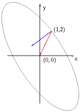
We assume the initial guess is ${\bf x}_0=[1,\;2]^T$, at which the gradient is ${\bf g}_0=[4,\;3]^T$. Now we compare the gradient method with Newton's method, in terms of the search direction ${\bf d}$ and progress of the iterations:

• Newton's method: Here we have

  $${\bf g}=\left[\begin{array}{c}2x_1+x_2\\ x_1+x_2\end{array}\right... ...ght],\;\;\;\; {\bf H}^{-1}=\left[\begin{array}{rr}1&-1\\ -1&2\end{array}\right]$$

  and the search direction is ${\bf d}_0=-{\bf H}^{-1}{\bf g}_0=-[1,\;2]^T$ (the red arrow in the figure). The iteration is:

  $${\bf x}_1={\bf x}_0-{\bf H}^{-1}{\bf g}_0=\left[\begin{array}{rr}... ...array}{r}4\\ 3\end{array}\right] =\left[\begin{array}{r}0\\ 0\end{array}\right]$$

  which is the minimum of the function.
• The gradient descent method: the search direction is ${\bf d}_0=-{\bf g}_0=-[4,\;3]^T$, perpendicular to the contour of the function. The first iteration is:

  $${\bf x}_1={\bf x}_0-\delta{\bf g}_0 =\left[\begin{array}{r}1\\ 2\... ...{array}\right] =\left[\begin{array}{r}1-\delta 4\\ 2-\delta 3\end{array}\right]$$

  We need to determine the step size $\delta$ (to be considered later) to find ${\bf x}_1$, and then continue the iteration.

The figure below shows the search direction of the Newton's method (red), which reaches the solution in a single step, based on not only the gradient ${\bf g}_0$, the local information at the point ${\bf x}_0$, but also the Hessian matrix ${\bf H}$, the global information of the quadratic function, in comparison to the gradient descent method (blue) based only on the local gradient ${\bf g}_0$. Without global information ${\bf H}$ representing the elliptical shape of the contour line of the quadratic function, the gradient descent method requires an iteration, and is therefore less effective.

In the gradient descent method, we also need to determine a proper step size $\delta$. If $\delta$ is too small, the iteration may converge too slowly, especially when $f(x)$ reduces slowly toward its minimum. On the other hand, if $\delta$ is too large but $f(x)$ has some rapid variations in the local region, the minimum of the function may be skipped and the iteration may not converge. We will consider how to find the optimal step size in the next section.