Newton-Raphson Method (Multivariate)

The Newton-Raphson method discussed above for solving a single-variable equation $f(x)=0$ can be generalized to the case of multivariate equation systems containing $M$ equations of $N$ variables in ${\bf x}=[x_1,\cdots,x_N]^T$:

$${\bf f}({\bf x})=\left[\begin{array}{c} f_1({\bf x}) \\ \vdots\\ ... ...nd{array}\right] =\left[\begin{array}{c}0\\ \vdots\\ 0\end{array}\right]={\bf0}$$ (95)

To solve the equation system, we first consider the Taylor series expansion of each of the $M$ functions in the neighborhood of the initial point ${\bf x}_0=[x_{01},\cdots,x_{0N}]^T$:

$$f_m({\bf x}) =f_m({\bf x}_0)+\sum_{n=1}^N\frac{\partial f_m({\bf ... ...) +r_m(\vert\vert{\bf x}-{\bf x}_0\vert\vert^2), \;\;\;\;\;\;\;\;(m=1,\cdots,M)$$ (96)

where $r_m(\vert\vert{\bf x}-{\bf x}_0\vert\vert^2)$ represents the second and higher order terms in the series beyond the linear term, which can be neglected if $\vert\vert{\bf x}-{\bf x}_0\vert\vert$ is small. These $M$ equations can be expressed in matrix form

$${\bf f}({\bf x}) = \left[\begin{array}{c}f_1({\bf x})\\ \vdots\\ f_M({\bf x})\end{ar... ...\end{array}\right] +\left[\begin{array}{c}r_1\\ \vdots \\ r_M\end{array}\right]$$

$$= {\bf f}({\bf x}_0)+{\bf J}({\bf x}_0)\;({\bf x}-{\bf x}_0)+{\bf r... ..._0)+{\bf J}({\bf x}_0)\;({\bf x}-{\bf x}_0) ={\bf f}_0+{\bf J}_0\;\Delta{\bf x}$$ (97)

where $\Delta{\bf x}={\bf x}-{\bf x}_0$, while ${\bf f}_0={\bf f}({\bf x}_0)$ and ${\bf J}_0={\bf J}({\bf x}_0)$ are the function ${\bf f}({\bf x})$ and its Jacobian matrix ${\bf J}_f({\bf x})$ both evaluated at ${\bf x}_0$. We further consider solving the equation system ${\bf f}({\bf x})={\bf0}$ in the following two cases:

• $M=N$: The number of equations is the same as the number of unknowns, the Jacobian ${\bf J}({\bf x})$ is a square matrix and its inverse ${\bf J}^{-1}$ exists in general. In the special case where ${\bf f}({\bf x})$ is linear, the Taylor series contains only the first two terms while all higher order terms are zero, and the approximation in Eq. (97) becomes exact. To find the root ${\bf x}^*$ satisfying ${\bf f}({\bf x}^*)={\bf0}$, we set ${\bf f}({\bf x})$ in Eq. (97) to zero and solve the resulting equation for ${\bf x}$ to get

  $${\bf x}^*={\bf x}={\bf x}_0-{\bf J}_0^{-1}{\bf f}_0 ={\bf x}_0-{\bf A}^{-1}{\bf f}_0$$ (98)

  As in general ${\bf f}({\bf x})$ is nonlinear, it can only be approximated by the first two terms of the Taylor series, consequently the result above is only an approximation of the optimal solution. But this approximation can be improved iteratiively to approach the optimal solution ${\bf x}^*$:

  $${\bf x}_{n+1}={\bf x}_n+\Delta {\bf x}_n ={\bf x}_n-{\bf J}_n^{-1}\;{\bf f}_n$$ (99)

  where we have defined $\Delta {\bf x}_n=-{\bf J}_n^{-1}\;{\bf f}_n$ as the increment, which can also be denoted by ${\bf d}_n=\Delta{\bf x}_n$ to represent the search or Newton direction. The iteration moves ${\bf x}_n$ in the N-D space spanned by $\{x_1,\cdots,x_N\}$ from some initial guess ${\bf x}_0$ along such a path that all function values $f_m({\bf x}),\;\;m=1,\cdots,M$) are reduced. Same as in the univariate case, a scaling factor $\delta_n$ can be used to control the step size of the iteration

  $${\bf x}_{n+1}={\bf x}_n+\delta_n\,\Delta{\bf x}_n ={\bf x}_n-\delta_n\,{\bf J}_n^{-1}\; {\bf f}_n$$ (100)

  When $\delta<1$, the step size becomes smaller and the convergence of the iteration is slower, however, we will have a better chance not to skip a solution, which may happen if ${\bf f}({\bf x})$ is not smooth and the step size is too big.

  The algorithm is listed below:

  • Select ${\bf x}_0$
  • Obtain ${\bf f}_0={\bf f}({\bf x}_0)$ and ${\bf J}_0$
  • Obtain ${\bf J}_0^{-1}$
  • $n=0$
  • While $\vert\vert{\bf x}_{n+1}-{\bf x}_n\vert\vert> tol$ do
    • ${\bf x}_{n+1}={\bf x}_n-{\bf J}_n^{-1}{\bf f}_n$
    • Find ${\bf f}_{n+1}$ and ${\bf J}_{n+1}$
    • $n=n+1$

• $M>N$: There are more equations than unknowns, i.e., equation ${\bf f}({\bf x})={\bf0}$ is an over-constrained system, and the Jacobian ${\bf J}({\bf x})$ is an $M\times N$ non-square matrix without an inverse, i.e., no solution exists for the equation ${\bf f}({\bf x})={\bf0}$ in general. But we can still seek to find an optimal solution ${\bf x}^*$ that minimizes the following sum-of-squares error:

  $$\varepsilon({\bf x})=\frac{1}{2}\vert\vert{\bf f}({\bf x})\vert\v... ...1}{2}{\bf f}({\bf x})^T{\bf f}({\bf x}) =\frac{1}{2}\sum_{m=1}^M f_m^2({\bf x})$$ (101)

  The gradient vector of $\varepsilon({\bf x})$ is:

  $${\bf g}_\varepsilon({\bf x}) =\frac{d}{d{\bf x}}\varepsilon({\bf ... ..._m^2({\bf x})\right) =\sum_{m=1}^M \frac{d}{d{\bf x}}f_m({\bf x})\;f_m({\bf x})$$ (102)

  The nth component of ${\bf g}_\varepsilon({\bf x})$ is

  $$\frac{\partial\varepsilon({\bf x})}{\partial x_n} =\sum_{m=1}^M \... ... x_n}\;f_m({\bf x}) =\sum_{m=1}^M J_{mn}\;f_m({\bf x}) \;\;\;\;\;(n=1,\cdots,N)$$ (103)

  where $J_{mn}=\partial f_m({\bf x})/\partial x_n$ is the component in the mth row and nth column of the Jacobian matrix ${\bf J}_f({\bf x})$ of ${\bf f}({\bf x})$. Now the gradient can be written as

  $${\bf g}_{\varepsilon}({\bf x})={\bf J}^T_f({\bf x})\,{\bf f}({\bf x})$$ (104)

  If ${\bf f}({\bf x})$ is linear and can therefore be represented as the sum of the first two terms of its Taylor series in Eq. (97), then the gradient is:

  $${\bf g}_{\varepsilon}({\bf x})={\bf J}^T({\bf x})\,{\bf f}({\bf x... ...bf J}({\bf x}_0)\Delta {\bf x}] ={\bf J}_0^T( {\bf f}_0+{\bf J}_0\Delta{\bf x})$$ (105)

  where ${\bf x}_0$ is any chosen initial guess. If we assume ${\bf x}$ is the optimal solution at which $\varepsilon({\bf x})$ is minimized and ${\bf g}_{\varepsilon}({\bf x})$ is zero:

  $${\bf g}_{\varepsilon}({\bf x}) ={\bf J}_0^T({\bf f}_0+{\bf J}_0\Delta{\bf x})={\bf0}$$ (106)

  then the increment $\Delta{\bf x}$ can be found by solving the equation

  $$\Delta{\bf x}=-({\bf J}^T_0{\bf J}_0)^{-1}{\bf J}^T_0{\bf f}_0 =-{\bf J}_0^-\,{\bf f}_0$$ (107)

  Here ${\bf J}_0^-=({\bf J}^T_0{\bf J}_0)^{-1}{\bf J}^T_0$ is the pseudo-inverse of the non-square matrix ${\bf J}_0$. Now the optimal solution can be found as:

  $${\bf x}^*={\bf x}_0+\Delta{\bf x}={\bf x}_0-{\bf J}_0^-\,{\bf f}_0$$ (108)

  However, as ${\bf f}({\bf x})$ is nonlinear in general, the sum of the first two terms of its Taylor series is only an approximation. Consequently the result ${\bf x}={\bf x}_0+\Delta{\bf x}$ above is not the optimal solution, but an estimate which can be improved by carrying out this step iteratively:

  $${\bf x}_{n+1}={\bf x}_n+\Delta{\bf x}_n ={\bf x}_n-{\bf J}_n^-\; {\bf f}_n$$ (109)

  This iteration will converge to ${\bf x}^*$ at which ${\bf g}_\varepsilon({\bf x}^*)={\bf0}$, and the squared error $\varepsilon({\bf x})$ is minimized.

  Specially, for a linear equation system ${\bf f}({\bf x})={\bf Ax}-{\bf b}={\bf0}$, the Jacobian is simplely ${\bf J}_f({\bf x}_n)={\bf A}$, and the optimal solution is

  $${\bf x}_{n+1}={\bf x}_n-{\bf A}^-{\bf f}_n ={\bf x}_n-({\bf A}^T{... ...T({\bf Ax}_n-{\bf b}) =({\bf A}^T{\bf A})^{-1}{\bf A}^T{\bf b}={\bf A}^-{\bf b}$$ (110)

  i.e., the optimal solution can be found from any initial guess in a single step. This result is the same as that in Eq. (7).

Comparing Eqs. (99) and (109), we see that the two algorithms are essentially the same, with the only difference that the regular inverse ${\bf J}^{-1}$ is used when $M=N$, but the pseudoinverse ${\bf J}^-$ is used when $M>N$ and ${\bf J}^{-1}$ does not exist.

The Newton-Raphson method assumes the availability of the analytical expressions of all partial derivatives $J_{mn}=\partial f_m({\bf x})/\partial x_n\;(m=1,\cdots,M,\;n=1,\cdots,N)$ in the Jacobian matrix ${\bf J}$. However, when this is not the case, $J_{mn}$ need to be approximated by forward or central difference (secant) method:

$$J_{mn}=\frac{\partial f_m(x_1,\cdots,x_N)}{\partial x_n} \approx \frac{f_m(x_1,\cdots,x_n+h,\cdots,x_N) -f_m(x_1,\cdots,x_n,\cdots,x_N)}{h}$$

$$\approx \frac{f_m(x_1,\cdots,x_n+h,\cdots,x_N) -f_m(x_1,\cdots,x_n-h,\cdots,x_N)}{2h}$$ (111)

where $h$ is a small increment.

Example 1

$$\left\{ \begin{array}{l} 3 \,x_1-\cos(x_2 x_3)-3/2=0\\ 4x_1^... ...,x_2^2+2 x_3-1=0\\ 20 \,x_3+e^{-x_1x_2}+9=0 \end{array}\right.$$

$${\bf J}=\left[ \begin{array}{ccc} 3 & x_3\sin(x_2 x_3) & x_2\... ...x_2\,e^{-x_1 x_2} & -x_1\,e^{-x_1 x_2} & 20 \end{array} \right]$$

$$\begin{array}{c\vert c\vert c}\hline n & {\bf x} & error \\ \... ....833282, 0.035335, -0.498549) & 5.551e-16 \\ \hline \end{array}$$

Example 2

$${\bf f}({\bf x})={\bf0},\;\;\;\;\;\;\;\;\;\; \left\{ \begin{array... ...+x_2x_3+2=0\\ f_3({\bf x})=x_1x_3^2-3x_3+x_2x_3^2+x_1x_2=0 \end{array} \right.$$

$${\bf J}=\left[\begin{array}{ccc} 2x_1-2 & 2x_2 & -1\\ x_2^2-1 & ... ..._2-3+x_3 & x_2 \\ x_3^2+x_2 & x_3^2+x_1 & 2x_1x_3-3+2x_2x_3 \end{array}\right]$$

With ${\bf x}_0=[1,\;2,\;3]^T$, we get a root:

$$\begin{array}{c\vert c\vert c}\hline n & {\bf x} & error \\ \... ...& (1.00000, 1.00000, 1.00000) & 6.701e-06 \\ \hline \end{array}$$

With ${\bf x}_0=[0,\;0,\;0]^T$, we get another root:

$$\begin{array}{c\vert c\vert c}\hline n & {\bf x} & error \\ \... ...& (1.09888, 0.36764, 0.14494) & 4.817e-06 \\ \hline \end{array}$$

Broyden's method

In the Newton-Raphson method, two main operations are carried out in each iteration: (a) evaluate the Jacobian matrix ${\bf J}_{\bf f}({\bf x}_n)$ and (b) obtain its inverse ${\bf J}^{-1}_{\bf f}({\bf x}_n)$. To avoid these expensive computation for these operations, we can consider using Broyden's method, one of the quasi-Newton methods, which approximates the inverse of the Jacobian ${\bf J}^{-1}_{n+1}={\bf J}^{-1}({\bf x}_{n+1})$ from the ${\bf J}^{-1}_n={\bf J}^{-1}({\bf x}_n)$ in the previous iteration step, so that it can be updated iteratively from the initial ${\bf J}^{-1}_0={\bf J}^{-1}({\bf x}_0)$.

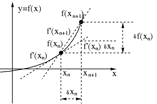
We first consider in the single-variable case how to estimate the next derivative $f'_{n+1}=f'(x_{n+1})$ from the current $f'_n=f'(x_n)$ by the secant method:

$$f'_{n+1}\approx \hat{f}'_{n+1} = \frac{f_{n+1}-f_n}{x_{n+1}-x_n} =\frac{\delta f_n}{\delta x_n} =\frac{\hat{f}'_n\delta x_n-\hat{f}'_n\delta x_n+\delta f_n}{\delta x_n}$$

$$= \hat{f}'_n+\frac{\delta f_n-\hat{f}'_n\delta x_n}{\delta x_n} =\hat{f}'_n+\hat{\delta} f'_n$$ (112)

where

• $\delta f_n=f_{n+1}-f_n$ is the true increment of the function over the interval $\delta x_n=x_{n+1}-x_n$;
• $\hat{f}'_n\delta x_n$ is the estimated increment of the function based on the previous derivate $\hat{f}'_n$;
• $\hat{\delta}f'_n$ is the estimated increment of the derivative:

  $$\hat{\delta}f'_n=\frac{\delta f_n-\hat{f}'_n\delta x_n}{\delta x_n}$$ (113)

The equation above indicates that the derivative $f'_{n+1}$ in the $(n+1)th$ step can be estimated by adding the estimated increment $\hat{\delta}f'_n$ to the derivative $\hat{f}'n$ in the current $nth$ step.

Having obtained $\hat{f}'_{n+1}$, we can use the same iteration in the Newton-Raphson method to find $x_{n+1}$:

$$x_{n+1}=x_n-\frac{f(x_n)}{\hat{f}'_n}$$ (114)

This method for single-variable case can be generalized to multiple variable case for solving ${\bf f}({\bf x})={\bf0}$. Following the way we estimate the increment of the derivative of a single-variable function in Eq. (113), here we can estimate the increment of the Jacobian of a multi-variable function:

$$\delta\hat{\bf J}_n =\frac{(\delta{\bf f}_n-\hat{{\bf J}}_n\delta... ...J}}_n\delta{\bf x}_n)\delta{\bf x}^T_n}{\vert\vert\delta {\bf x}_n\vert\vert^2}$$ (115)

where $\delta{\bf x}_n={\bf x}_{n+1}-{\bf x}_n$ and $\delta{\bf f}_n={\bf f}_{n+1}-{\bf f}_n={\bf f}({\bf x}_{n+1})-{\bf f}({\bf x}_n)$. Now in each iteration, we can update the estimated Jacobian as well as the estimated root:

$$\hat{\bf J}_{n+1}=\hat{\bf J}_n+\delta\hat{\bf J}_n,\;\;\;\;\;\;\... ...}={\bf x}_n+\delta {\bf x}_n ={\bf x}_n-\hat{{\bf J}}_n^{-1} {\bf f}({\bf x}_n)$$ (116)

The algorithm can be further improved so that the inverse of the Jacobian ${\bf J}_n$ is avoided. Specifically, consider the inverse Jacobian:

$$\hat{{\bf J}}_{n+1}^{-1}=\left( \hat{{\bf J}}_n+\delta\hat{\bf J}... ...bf x}_n)\delta{\bf x}^T_n}{\vert\vert\delta {\bf x}_n\vert\vert^2} \right]^{-1}$$ (117)

We can apply the Sherman-Morrison formula:

$$({\bf A}+{\bf u}{\bf v}^T)^{-1} ={\bf A}^{-1}-\frac{{\bf A}^{-1}{\bf u}{\bf v}^T{\bf A}^{-1}} {1+{\bf v}^T{\bf A}^{-1}{\bf u}}$$ (118)

to the right-hand side of the equation above by defining

$${\bf A}=\hat{\bf J}_n,\;\;\;\;\;\;\; {\bf u}=\frac{\delta{\bf f}_... ...}{\vert\vert\delta{\bf x}_n\vert\vert^2}, \;\;\;\;\;\;\;{\bf v}=\delta{\bf x}_n$$ (119)

and rewrite it as:

$$\hat{{\bf J}}^{-1}_{n+1}=\hat{{\bf J}}^{-1}_n\,-\,\frac{\hat{{\bf... ...n\,\hat{{\bf J}}_n^{-1}} {\delta{\bf x}^T_n\hat{{\bf J}}_n^{-1}\delta{\bf f}_n}$$ (120)

We see that the next $\hat{\bf J}_{n+1}^{-1}$ can be iteratively estimated directly from the previous $\hat{\bf J}_n^{-1}$, thereby avoiding computing the inverse of $\hat{\bf J}_n$ altogether. The algorithm is listed below:

• Select ${\bf x}_0$
• Find ${\bf f}_0={\bf f}({\bf x}_0)$, ${\bf J}_0={\bf J}({\bf x}_0)$, and ${\bf J}_0^{-1}$
• ${\bf x}_1={\bf x}_0-{\bf J}_0^{-1}{\bf f}_0$
• $n=0$
• While $\vert\vert{\bf x}_{n+1}-{\bf x}_n\vert\vert> tol$ do
  • $\delta{\bf x}_n={\bf x}_{n+1}-{\bf x}_n$
  • ${\bf f}_{n+1}={\bf f}({\bf x}_{n+1})$
  • $\delta{\bf f}={\bf f}_{n+1}-{\bf f}_n$
  • ${\bf J}_n^{-1}={\bf J}_n^{-1}-(\delta{\bf x}_n-{\bf J}_n^{-1}\delta{\bf f}_n) \delta{\bf x}_n^T{\bf J}_n^{-1}/(\delta{\bf x}_n^T{\bf J}_n^{-1}\delta{\bf f}_n)$
  • ${\bf x}_n={\bf x}_{n+1}$, ${\bf f}_n={\bf f}_{n+1}$
  • ${\bf x}_{n+1}={\bf x}_n-{\bf J}_n^{-1}{\bf f}_n$
  • $n=n+1$