Bias-Variance Tradeoff and Ridge Regression

In a generic regression problem, the goal is to estimate the unknown relationship $y=f({\bf x})$ between the dependent variable $y$ and the $d$ independent variables ${\bf x}=[x_1,\cdots,x_d]^T$, by a model function $\hat{f}({\bf x})$, based on a set of given training data ${\cal D}=\{({\bf x}_n,\,y_n)\;n=1,\cdots,N\}$, contaminated by some rero-mean random noise $e$ with variance $\sigma^2$:

$$y=f({\bf x})+e,\;\;\;\;\;\;\; E[e]=0,\;\;\;\; \Var[e]=E[(e-E[e]^2)]=E[e^2]=\sigma^2$$ (136)

As a function of the random training samples ${\bf x}$, the estimated function $\hat{f}({\bf x})$ is also random, and, by assumption, it is independent of $e$, i.e., $p(e\,\hat{f})=p(e)\;p(\hat{f})$, therefore $E[e\,\hat{f}]=E[e]\,E[\hat{f}]$.

How well the model $\hat{f}({\bf x})$ fits the training data can be measured by the mean of its squared error (SE) defined as $[y-\hat{f}({\bf x})]^2$, called the mean squared error (MSE):

$$\E [ (y-\hat{f})^2 ] = \E[(f+e-\hat{f})^2 ] =\E\left[ [ (f-E\hat{f})+(E\hat{f}-\hat{f})+e]^2 \right]$$

$$= E\left[ (f-E\hat{f})^2+(E\hat{f}-\hat{f})^2+e^2 +2 [e(f-E\hat{f})+e(E\hat{f}-\hat{f}) +(f-E\hat{f})(E\hat{f}-\hat{f}) ]\right]$$

$$= \E[(f-E\hat{f})^2]+\E[(E\hat{f}-\hat{f})^2]+E (e^2)$$

$$+ 2\E[ e(f-E\hat{f}) ] +2\E[e(E\hat{f}-\hat{f})] +2\E[(E\hat{f}-\hat{f})(f-E\hat{f})]$$

$$= \E[(f-E\hat{f})^2]+\E[(E\hat{f}-\hat{f})^2]+\E[e^2]$$ (137)

The last equality is due to the fact that all three cross terms are zero:

$$\left\{ \begin{array}{l} \E[e(f-E\hat{f})]=\E[e]\;\E[f-E\hat{f}]=... ...t{f}-\hat{f})(f-E\hat{f})]=(E\hat{f}-E\hat{f})(f-E\hat{f})=0 \end{array}\right.$$ (138)

The three remaining terms represent three different types of error:

• Irreducible Error $\E[e^2]=\sigma^2$, due to the inevitable observation error.

• Bias Error: $\E[(f-E\hat{f})^2]=(f-E\hat{f})^2$, the squared bias, the difference between the estimated function and the true function, measuring how well the estimated function $\hat{f}$ based on the training data models the true function $f$;

• Variance Error: $\E[\hat{f}-E\hat{f}]^2=\Var[\hat{f}]$, the variance of the estimated function $\hat{f}$, measuring the variation of the model due to the noise in the training data.

We therefore get the following general relationship in terms of the three types of error:

$$= + +$$ (139)

In the noise-free case with $E(e^2]=0$, we have:

$$= +$$ (140)

The variance error and bias error are illustrated below:

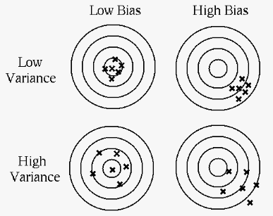
Given the total MSE and the irreducible error $\sigma^2$, the bias error and the variance error are complementary, i.e., if one error is higher, the other is lower, depending on the model function $\hat{f}$ produced by the specific algorithm. This is called the bias-variance tradoff, which is related to the major issur of overfitting vs. underfitting in supervised learning:

• Overfitting: In order to fit the training data closely so that the detailed variations cuased by noise are to be matched, it may be necessary to use a complex model, which tends to have low bias error, but may suffer from high variance error as it may be overly affected by the random noise (possibly some outliers) and does not generalize well accross datasets contaminated by varying noise.

• Underfitting: In order not to be overly affected by the random noise, a simple model can be used without matching the training data very closely. Such a model tends to have low variance error as it is insensitive to the varying random noise accross datasets, but it may suffer from high bias error as it may not fit the signal variations.

$$\begin{tabular}{l\vert\vert c\vert c}\hline & Overfit & Underfit ... ...ce error & High & Low \\ \hline Bias error & Low & High \\ \hline \end{tabular}$$ (141)

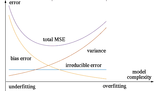
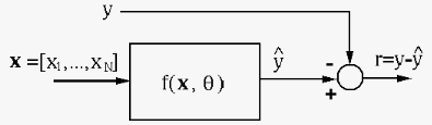
As both overfitting and underfitting result in poor predicttion capability, they need to be avoided by making a proper tradeoff between bias-error/underfitting and variance-error/overfitting. This is an important issue not only in the context of regression, but also in general in all supervised learning algorithms, for the purpose of predicting either a value as in regression, or a categorical class in classification, based on the output $\hat{y}=f({\bf x})$ as a function of the given data point ${\bf x}$. A general framework for all such algorithms is shown below, where the algorithm in the box is to come up with a model function $f({\bf x},{\bf\theta})$ of which the output $\hat{y}$ need to match the labeling $y$ of the data point ${\bf x}$ in some optimal way:

Due to the inevitable noise in the training data, all such algorithms face the same issue of how to make a proper tradeoff between overfitting and underfitting, as illustrated below.

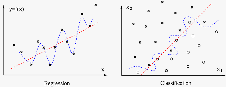
We see that in regression on the left, a set of data points is modeled by two different regression functions, while in classification on the right, the 2-D space is partitioned into two regions corresponding to two classes by two different decision boundaries. The issue is, which of the two models, in either regression or classification, fits the data better, in terms of underfitting versus overfitting.

• Underfitting:

  The simple linear regression function or decision boundary (red) may underft the data as it may miss some legitimate variations in the data.

• Overfitting:

  The complex regression model, e.g., a high order polynomial, or decision boundary (blue) may overfit the data as it may be overly affected by the variation due to the observation noise.

In general, based on a single set of training data points, it is impossible to distinguish between signal and random noise, and to judge whether a learning algorithm over or underfits the data. However, based on multiple datasets contaminated by different random noise, overfitting problem can be detected if the algorithm produces significantly different results when trained by different datasets. Based on this idea, the method of cross-validation can be used to train a learning algorithm by a subset of the training dataset and then test the algorithm by a different subset of the data. if the residual error during testing is large, then the algorithm may suffer from overfitting.

Many regression and classification algorithms address the issue of overfitting versus underfitting by a process called regularization to prevent overfitting, espeicially when the problem is ill-conditioned, so that the model is less sensitive to noise in the training data and therefore more generalizable, while still able to capture the essential nature and behavior of the signal. Typically this is done by adjusting some hyperparameter of the model to make a proper tradeoff between the two extremes of over and underfitting.

As an exammple, consider the method of ridge regression for LS linear regression. If the $N$ data points in the training set are barely independent, then matrix ${\bf XX}^T$ has full rank but is very close to singularity, and its smallest eigenvalue $\lambda_{min}$, the smallest singular value $\sigma_{min}=\sqrt{\lambda_{min}}$ of ${\bf A}$, is close to zero, and the normal equation ${\bf XX}^T{\bf w}={\bf Xy}$ (Eq. (115)) is ill-conditioned. Now the solution ${\bf w}=({\bf X}^T)^-{\bf y}$ based on the pseudo-inverse is unstable and prone to noise. Any minor change due to noise in the dataset (in either ${\bf X}$ or ${\bf y}$) may cause a huge change in ${\bf w}$, i.e., the resulting ${\bf w}$ has a large variance error and the regression model overfits the data and is therefore poor generalizable.

In this case, the ridge regression method can be used to regularize the ill-conditioned problem by constructing an objective function $J({\bf w})$ that contains a regularization or penalty term $\lambda\vert\vert{\bf w}\vert\vert^2/2$ to discourage large weights while minimizing the error $\varepsilon=\vert\vert{\bf r}\vert\vert^2/2$:

$$J({\bf w})=\frac{1}{2}\vert\vert{\bf y}-{\bf X}^T{\bf w}\vert\vert^2 +\frac{\lambda}{2}\vert\vert{\bf w}\vert\vert^2$$ (142)

This method is in general call weight decay and the hyperparameter $\lambda$ is called the weight decay parameter. Solving the equation

$$\frac{d}{d{\bf w}} J({\bf w}) ={\bf XX}^T{\bf w}-{\bf Xy}+\lambda{\bf w} =({\bf XX}^T+\lambda{\bf I}){\bf w}-{\bf Xy} ={\bf0}$$ (143)

we get

$${\bf w}^*=({\bf XX}^T+\lambda{\bf I})^{-1}{\bf Xy}$$ (144)

Now a proper tradeoff between accuracy and stability can be made by adjusting the hyperparameter $\lambda$:

• Small $\lambda$: the solution is more accurate but also more prone to noise and therefore less stable, i.e., large variance error but small bias error, or overfitting;
• Large $\lambda$: the solution is more stable as it is less affacted by noise, but it may be less accurate, i.e., small variance error but large bias error, or underfitting.