Second Order Systems

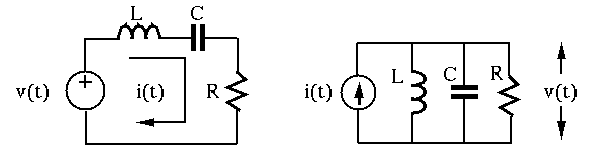
• The RCL series circuit (left) with an input $v(t)$ and output $i(t)$ is described by the following equation:

  $$v_R(t)+v_L(t)+v_C(t)=R\,i(t)+L\frac{di(t)}{dt}+\frac{1}{C}\int i(t) dt=v_s(t)$$ (166)

  Taking derivative and dividing by $L$ on both sides we get a 2nd-order linear constant coefficient differential equation (LCCDE):

  $$i''(t)+\frac{R}{L}\,i'(t)+\frac{1}{LC}\,i(t)=\frac{1}{L} v'_s(t)$$ (167)

  Alternatively, as $i(t)=C dv_C(t)/dt$, we have

  $$v_R(t)=R\;i(t)=R\,C\frac{d\,v_C(t)}{dt},\;\;\;\;\;\; v_L(t)=L\fra... ...t)=L\frac{d}{dt}\left[C\frac{d\,v_C(t)}{dt} \right] =LC\frac{d^2\,v_C(t)}{dt^2}$$ (168)

  the equation above can be written as a 2nd order ODE in terms of $v_C(t)$:

  $$v''_C(t)+\frac{R}{L} v'_C(t)+\frac{1}{LC}v_C(t)=\frac{1}{LC}v_s(t)$$ (169)

• The RCL parallel circuit (right) with input $i(t)$ and output $v(t)$ is described by the following equation:

  $$i_R(t)+i_C(t)+i_L(t)=\frac{v(t)}{R}+C\frac{dv(t)}{dt}+\frac{1}{L}\int v(t)\;dt =i_s(t)$$ (170)

  Taking derivative and dividing by $C$ on both sides we get a 2nd-order LCCDE:

  $$v''(t)+\frac{1}{RC}\,v'(t)+\frac{1}{LC}\,v(t)=\frac{1}{C}i'_s(t)$$ (171)

• Other RCL circuits (not pure series or parallel):

  

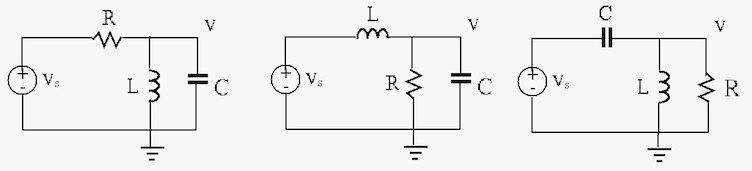
  $$\frac{v_s-v}{R} = C\frac{dv}{dt}+\frac{1}{L} \int v\;dt, \;\;\;\;... ...{dv}{dt}, \;\;\;\;\; C\frac{d}{dt} (v_s-v) = \frac{v}{R}+\frac{1}{L} \int v\;dt$$ (172)

  $$v''+\frac{1}{RC} v'+\frac{1}{LC}v=\frac{v'_s}{RC}, \;\;\;\;\;\;\;... ...1}{LC}v=\frac{1}{LC}v_s, \;\;\;\;\;\;\; v''+\frac{1}{RC} v'+\frac{1}{LC}v=v''_s$$ (173)

The dimensionality of the coefficient of the first order term is frequency:

$$\left[\frac{R}{L}\right]=\frac{[V][/[I]}{[VT]/[I]}=\frac{1}{[T]},... ...;\;\; \left[\frac{1}{RC}\right]=\frac{[I]}{[V]}\frac{[V]}{[I][T]}=\frac{1}{[T]}$$ (174)

The dimensionality of the coefficient of the constant terms is frequency squared:

$$\left[\frac{1}{LC}\right]=\frac{1}{[VT]/[I]\;[IT]/[V]}=\frac{1}{[T]^2}$$ (175)

In general, any 2nd-order LCCDE with input $x(t)$ and output $y(t)$ can be written in the canonical form

$$y''(t)+2\zeta\omega_n\,y'(t)+\omega_n^2\, y(t)= x(t)$$ (176)

in terms of the two parameters:

• damping coefficient $\zeta$ (unitless)
• natural frequency $\omega_n$ (frequency)

Comparing the canonical form with two equations above we see that for both RLC series and parallel circuits:

$$\omega_n=\frac{1}{\sqrt{LC}}$$ (177)

and

• for RLC series circuit

  $$\frac{R}{L}=2\zeta_s\omega_n=2\zeta_s\frac{1}{\sqrt{LC}},\;\;\;\; \;\;\;\;\; \zeta_s=\frac{R}{2}\sqrt{\frac{C}{L}}$$ (178)

• for RLC parallel circuit

  $$\frac{1}{RC}=2\zeta_p\omega_n=2\zeta_p\frac{1}{\sqrt{LC}}, \;\;\;\;\; \;\;\;\;\; \zeta_p=\frac{1}{2R}\sqrt{\frac{L}{C}}$$ (179)

We also have:

$$\zeta_p \zeta_s=\frac{1}{4},\;\;\;\;\;\zeta_p=\frac{1}{4\zeta_s}, \;\;\;\;\;\zeta_s=\frac{1}{4\zeta_p}$$ (180)

Note the following dimensionalities:

$$\left[\sqrt{\frac{L}{C}}\right]=\sqrt{\frac{[Henry]}{[Farad]}} =\... ...nd]}{[Ampere]}\frac{[Volt]}{[second]\;[Ampere]}} =\frac{[Volt]}{[Ampere]}=[Ohm]$$ (181)

$$\left[ \sqrt{LC} \right]=\sqrt{[Henry]\;[Farad]} =\sqrt{\frac{[Volt]\;[second]}{[Ampere]}\frac{[Ampere]\;[second]}{[Volt]}} =[second]$$ (182)

We therefore see that $\zeta_s$ and $\zeta_p$ are unitless, and the dimension of $\omega_n=1/\sqrt{LC}$ is $1/[second]$ as frequency.