We next consider the complete solution (composed of both homogeneous
and particular solutions) of the 2nd order DE
 |
(232) |
with a unit step  input and zero initial conditions
 . As the input is a constant for
  , we can
assume the particular solution to be a constant
, we can
assume the particular solution to be a constant  with zero
derivatives
with zero
derivatives
 . Substituting these into the DE above,
we get
. Substituting these into the DE above,
we get
 , i.e., the steady state solution is:
 |
(233) |
The complete response can be obtained as the sum of the homogeneous
solution (same as that obtained previously) and particular solution,
corresponding to the transient and steady state response, respectively:
 |
(234) |
The two coefficients  and
and  can be obtained based on the two
zero initial conditions:
can be obtained based on the two
zero initial conditions:
Solving these equations we get:
 |
(236) |
Now the complete solution becomes:
![$\displaystyle y(t)=\frac{1}{\omega_n^2}\left[1-\left(\frac{s_2e^{s_1t}}{s_2-s_1...
...ht]
=\frac{1}{\omega_n^2}\left(1-\frac{s_2e^{s_1t}-s_1e^{s_2t}}{s_2-s_1}\right)$](img670.svg) |
(237) |
Alternatively, the nonhomogeneous 2nd-order LCCODE given above can
be converted into a 1st-order ODE system and solving which we obtain
the same results, as shown
here.
The two roots  and
and  take different forms depending on
whether the discriminant
take different forms depending on
whether the discriminant
 is greater
or smaller than 0, i.e., whether
is greater
or smaller than 0, i.e., whether  is greater or smaller then 1.
Here we only consider the case when
is greater or smaller then 1.
Here we only consider the case when
 , i.e.,
  ,
for an under-damped second order system. The two roots are
,
for an under-damped second order system. The two roots are
 and and |
(238) |
where  is the damped natural frequency:
 |
(239) |
Finally the complete solution of the non-homogeneous DE is:
where
 and and |
(241) |
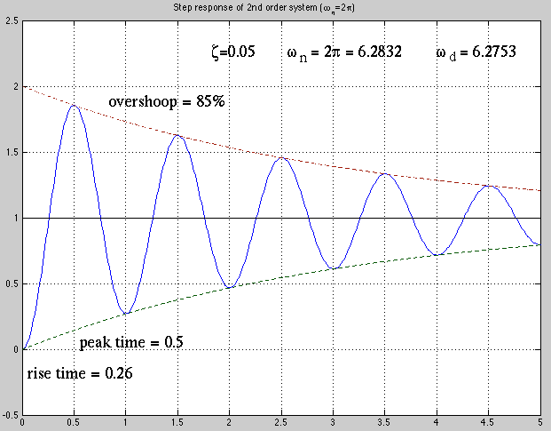
The step response  can be characterized by two parameters:
- Rise time:
The rise time  is the time at which reaches
  of the
steady state value
of the
steady state value  (assumed to be 1 for simplicity):
 or or |
(242) |
i.e.,
 or or |
(243) |
Solving for we get
 |
(244) |
But as
 , taking arctangent
on both sides we get
, taking arctangent
on both sides we get
 i.e. i.e. |
(245) |
- Peak time:
The peak time  is the time at which reaches the first peak, which can be
found by setting the time derivative of to zero, yielding
is the time at which reaches the first peak, which can be
found by setting the time derivative of to zero, yielding
 |
(246) |
i.e.,
 |
(247) |
or
 |
(248) |
We get
 for the first peak, i.e.,
 |
(249) |
Substituting inito we get the peak value:
The overshoot is
 .
.
In particular, if  and therefore
  , we have
![$\displaystyle y(t)=\frac{1}{\omega_n^2}\left[1-\sin(\omega_n t+\pi/2)\right]
=\frac{1}{\omega_n^2}\left[1-\cos(\omega_n t)\right]$](img705.svg) |
(251) |
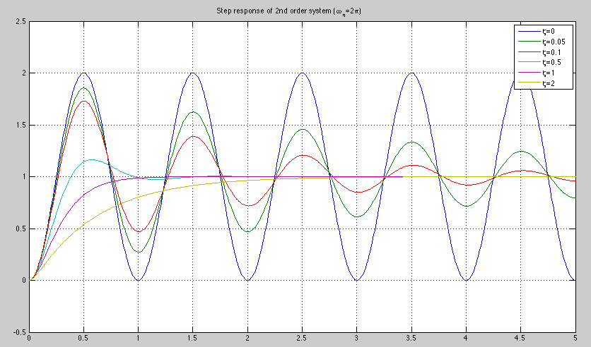
The plots below shows an example with
 . Note the critical
damped case when
. Note the critical
damped case when  . An overshoot will occur for any
  .
.
The step response is plotted below. Note that  and
and
 .
.
Example
Consider the response
 of an undamped 2nd order RCL system.
- Find the response of the RLC circuit to a step input
 .
The general solution is the sum of the homogeneous solution
.
The general solution is the sum of the homogeneous solution
 and the particular solution
  :
:
 |
(252) |
Consider two different sets of initial conditions:
- Find the system's response to a square impulse
 |
(255) |
As
 , the response is
![$\displaystyle y(t)=[1-\cos(\omega_nt)]u(t)-[1-\cos(\omega_n(t-t_0))]u(t-t_0)$](img724.svg) |
(256) |
When  , we have
 |
(257) |
We further consider two special cases.
- When
 , we have
This is a one period of a sinusoid.
- When
 , we have
This is a pure sinusoid after  .
.
- Find the impulse response
 . The input
  is an impulse which
can be written as
is an impulse which
can be written as
 |
(260) |
When
 , we have first order approximations
 and
and
 ,
and we get
,
and we get
 |
(261) |
Substituting this into
 we get the impulse response
 |
(262) |
- It is often desirable for a second order system to reach a set steady
state value without overshoot. This can be achieved by driving the system
by an impulse
 with response
 , followed
by a step
, followed
by a step  with response
![$\displaystyle [1-\cos(\omega_n(t-T/4))]u(t-T/4)=[1-\cos(\omega_nt-\pi/2)]u(t-T/4)
=[1-\sin(\omega_nt)]u(t-T/4)$](img746.svg) |
(263) |
The total response is
![$\displaystyle y(t)=\sin(\omega_nt)u(t)+[1-\sin(\omega_nt)]u(t-T/4)
=\left\{\begin{array}{cl} \sin(\omega_nt) & 0<t<T/4 \\
1 & t>T/4\end{array} \right.$](img747.svg) |
(264) |
We see that after reaches the first peak of  at
at  , it will
stay at the constant value as the two responses cancel each other for
, it will
stay at the constant value as the two responses cancel each other for
 .
.
- Alternatively, the steady state value
 can be achieved without
overshoot by applying an input
can be achieved without
overshoot by applying an input
![$x(t)=[u(t)-u(t-T/2)]/2$](img752.svg) . The response to
. The response to
 is
is
![$\displaystyle \frac{1}{2}[1-\cos(\omega_nt)]u(t)$](img754.svg) |
(265) |
while the response to
 is
is
![$\displaystyle \frac{1}{2}[1-\cos(\omega_n(t-T/2))]u(t-T/2)
=\frac{1}{2}[1-\cos(\omega_nt-\pi)]u(t-T/2)
=\frac{1}{2}[1+\cos(\omega_nt)]u(t-T/2)$](img756.svg) |
(266) |
The overall response is the difference between the two individual responses:
![$\displaystyle y(t)=\left\{\begin{array}{cl}
[1-\cos\omega_nt]/2 & 0<t<T/2 \\ 1 & t>T/2 \end{array} \right.$](img757.svg) |
(267) |
i.e., the response is  for all .
- It is desirable for a second order system to reach a steady state value
within a time delay
 without overshoot. We first consider
driving the system with a positive square pulse of value
without overshoot. We first consider
driving the system with a positive square pulse of value  followed
by a negative one of
followed
by a negative one of  :
:
![$\displaystyle x(t)=\left\{\begin{array}{cl}
V & (0<t<t_0/2) \\ (1-a)V & (t_0/2<t<t_0)
\end{array}\right. =V \left[u(t)-a u(t-t_0/2)\right]$](img762.svg) |
(268) |
The response for
 is:
is:
![$\displaystyle y(t)=V\left[ 1-\cos(\omega_nt)-a[1-\cos(\omega_n(t-t_0/2))]\right]$](img764.svg) |
(269) |
In order for the output to be a constant for , we need to
have the input  for , and set the initial conditions at
  to be
to be  and
and
 . To do so, we let
![$\displaystyle \frac{dy(t)}{dt}\bigg\vert _{t=t_0}=V\omega_n\left[ \sin(\omega_n...
...right]_{t=t_0}
=V\omega_n\left[ \sin(\omega_nt_0)-a\sin(\omega_nt_0/2)\right]=0$](img769.svg) |
(270) |
Based on the trigonometric identity
 , the equation above
can be written as
, the equation above
can be written as
 |
(271) |
Substituting this into the desired initial condition , we get
![$\displaystyle y(t_0)=V\left[ 1-\cos(\omega_nt_0)-2\cos(\omega_nt_0/2)
[1-\cos(\omega_n(t_0/2))]\right]
=2V(1-\cos(\omega_nt_0/2) =4V\sin^2(\omega_nt_0/4)=1$](img772.svg) |
(272) |
where we have used the trigonometric identities
 and
and
 . Solving this for we get
 |
(273) |
As now we have the initial conditions and
as
needed. If we set for , so that the output will be at
constant when .


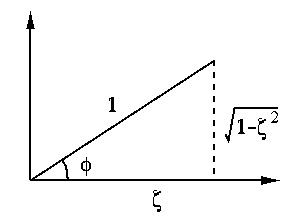
![$\displaystyle \frac{1}{\omega_n^2}\left[1-\left(\frac{s_2}{s_2-s_1}e^{s_1t}-\frac{s_1}{s_2-s_1}e^{s_2t}\right)\right]$](img677.svg)
![$\displaystyle \frac{1}{\omega_n^2}\left[ 1-
\left(\frac{\zeta+j\sqrt{1-\zeta^2}...
...1-\zeta^2}}{2j\sqrt{1-\zeta^2}} e^{(-\zeta\omega_n-j\omega_d)t} \right) \right]$](img678.svg)
![$\displaystyle \frac{1}{\omega_n^2}\left[ 1-\frac{e^{-\zeta\omega_nt}}{\sqrt{1-\...
...j\omega_dt}
-\frac{\zeta-j\sqrt{1-\zeta^2}}{2j} e^{-j\omega_dt} \right) \right]$](img679.svg)
![$\displaystyle \frac{1}{\omega_n^2}\left[ 1-\frac{e^{-\zeta\omega_nt}}{\sqrt{1-\...
...rac{ e^{j\phi} e^{ j\omega_dt}-e^{-j\phi} e^{-j\omega_dt} }{2j} \right) \right]$](img680.svg)
![$\displaystyle \frac{1}{\omega_n^2}\left[1-\frac{e^{-\zeta\omega_nt}}{\sqrt{1-\zeta^2}}
\sin(\omega_dt+\phi) \right]$](img681.svg)


 and
and
 , and
, and
![$\displaystyle y(t)=V+A\sin(\omega_nt)+B\cos(\omega_nt)=V[1-\cos(\omega_nt)]$](img716.svg)
 ,
,  . We have
 and
and
 and
and

![$\displaystyle [1-\cos(\omega_nt)]u(t)-[1-\cos(\omega_n(t-T))]u(t-T)$](img728.svg)

![$\displaystyle [1-\cos(\omega_nt)]u(t)-[1-\cos(\omega_n(t-T/2))]u(t-T/2)$](img731.svg)
![$\displaystyle [1-\cos(\omega_nt)]u(t)-[1+\cos(\omega_nt)]u(t-T/2)$](img732.svg)
