Homogeneous Solution

The homogeneous solution of the 2nd order DE can be found by solving the homogeneous equation:

$$y''(t)+2\zeta\omega_n y'(t)+\omega_n^2 y(t)=x(t)=0$$ (209)

where the right hand side of the DE for the input $x(t)=0$ is zero. Substituting the assumed solution $y(t)=Ae^{st}$ and its derivatives $\dot{y}(t)=s Ae^{st},\;y''(t)=s^2 Ae^{st}$ into the DE we get

$$(s^2+2\zeta\omega_n s+\omega_n^2)Ae^{st}=0$$ (210)

As we are not interested in a trivial solution, $Ae^{st}\ne 0$, and we get an algebraic equation

$$s^2+2\zeta\omega_n s+\omega_n^2=0$$ (211)

Solving this quadratic equation we get its two roots, the two eigenvalues of ${\bf A}$:

$$s_{1,2}=\left\{\begin{array}{ll} \left(-\zeta\pm\sqrt{\zeta^2-1}\... ...^2}\right)\omega_n=\omega_n e^{\mp j\phi} &\vert\zeta\vert< 1\end{array}\right.$$ (212)

where

$$\phi=\tan^{-1}\left(\frac{\sqrt{1-\zeta^2}}{\zeta}\right)$$ (213)

These two roots $s_{1,2}$ are either two real numbers or a pair complex conjugate numbers, depending on whether its discriminant is greater and smaller then 0:

$$\Delta=(2\zeta\omega_n)^2-4\omega_n^2=4\omega_n^2(\zeta^2-1) \lef... ...y}{ll}\ge 0 & \vert\zeta\vert\ge 1\\ < 0 & \vert\zeta\vert< 1\end{array}\right.$$ (214)

For a constant $\omega_n$ and a variable $\zeta$ that changes from $-\infty$ to $\infty$, the two roots $s_1$ (red) and $s_2$ (blue) can be represented as the root locus on the complex plane.

In particular, for the RCL circuit with all $R$, $C$, and $L$ values non-negative, we have $\zeta\ge 0$, i.e., we only need to consider the root locus on the left side of the complex plain.

Given the two roots $s_1$ and $s_2$, we can write the homogeneous solution as

$$y_h(t)=C_1 e^{s_1t}+C_2 e^{s_2t}$$ (215)

where the two coefficients $C_1$ and $C_2$ can be found based on the two initial conditions $y(0)$ and $y'(0)$. If we assume $\dot{y}(0)=0$ but $y(0)=y_0$, then we get

$$y(0) = y_h(t)\bigg\vert _{t=0}=C_1+C_2=y_0$$

$$\dot{y}(0) = \dot{y}_h(t)\bigg\vert _{t=0}=s_1C_1+s_2C_2=0$$ (216)

Solving these we get

$$C_1=\frac{s_2}{s_2-s_1} y_0,\;\;\;\;\;\;\;\;C_2=\frac{s_1}{s_1-s_2} y_0$$ (217)

and the homogeneous solution becomes:

$$y_h(t)=y_0 \left[ \frac{s_2 e^{s_1t}}{s_2-s_1}-\frac{s_1 e^{s_2t}}{s_2-s_1} \right] =\frac{y_0}{s_2-s_1} (s_2 e^{s_1t}-s_1 e^{s_2t})$$ (218)

Alternatively, the 2nd-order LCCODE in canonical form given above can also be solved if it is coverted into a 1st-order ODE system, as shown here.

The solution takes different forms depending on the value of the damping coefficient $\zeta$.

• Over-damped system ($\zeta>1$)
  

  $$y_h(t) = y_0 \left[ \frac{s_2 e^{s_1t}}{s_2-s_1}+\frac{s_1 e^{s_2t}}{s_1-s_2} \right]$$

  $$= y_0\left[\frac{-\zeta+\sqrt{\zeta^2-1}}{2\sqrt{\zeta^2-1}}e^{(-\z... ...qrt{\zeta^2-1}}{2\sqrt{\zeta^2-1}}e^{(-\zeta+\sqrt{\zeta^2-1})\omega_nt}\right]$$ (219)

  
  This is a sum of two exponentially decaying terms, without any overshoot or oscillation. Note that when $t=0$, $y_h=y_0$.

• Critically damped system ($\zeta=1$)

  Now we have

  $$s_1=s_2=-\omega_n=s$$ (220)

  and the homogeneous solution takes following form:
  

  $$y_h(t) = C_1 e^{st}+C_2 t e^{st}=C_1 e^{-\omega_nt}+C_2 t e^{-\omega_nt}$$

  $$\dot{y}_h(t) = \frac{d}{dt}[C_1 e^{st}+C_2 t e^{st}]=C_1se^{st}+C_2(e^{st}+ste^{st})$$ (221)

  
  Applying the initial conditions to this response we get
  

  $$y(0) = C_1=y_0$$

  $$\dot{y}(0) = s C_1+C_2=0$$ (222)

  
  Solving this we get if $s_1\ne s_2$:

  $$C_1=y_0, \;\;\;\;\;\;\;C_2=-sy_0=\omega_ny_0$$ (223)

  and the response is

  $$y_h(t)=C_1 e^{st}+C_2 t e^{st}=y_0\left[ e^{-\omega_nt}+\omega_n t e^{-\omega_nt}\right]$$ (224)

  Again, there is no overshoot or oscillation.
• Under-damped system ( $0 \le \zeta < 1$)

  $$s_{1,2}=(-\zeta\pm j \sqrt{1-\zeta^2})\omega_n=-\zeta\omega_n\pm j\omega_d, \;\;\;\; \;\;\;\; s_1-s_2=2j\omega_d$$ (225)

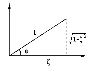
  where $\omega_d$ is the damped natural frequency defined as:

  $$\omega_d=\omega_n\sqrt{1-\zeta^2}$$ (226)

  The response is
  

  $$y_h(t) = y_0 \left[ \frac{s_2 e^{s_1t}}{s_2-s_1}+\frac{s_1 e^{s_2t}}{s_1-s_2} \right]$$

  $$= y_0\left[ \frac{(-\zeta-j\sqrt{1-\zeta^2})\omega_n}{-2j\omega_n\s... ...)\omega_n}{-2j\omega_n\sqrt{1-\zeta^2}} e^{(-\zeta\omega_n-j\omega_d)t} \right]$$

  $$= y_0\frac{e^{-\zeta\omega_nt}}{\sqrt{1-\zeta^2}} \left(\frac{e^{j\... ...j}\right) =y_0\frac{e^{-\zeta\omega_nt}}{\sqrt{1-\zeta^2}} \sin(\omega_dt+\phi)$$ (227)

  
  Here we have defined:

  $$\phi=\tan^{-1}\left( \frac{\sqrt{1-\zeta^2}}{\zeta} \right),\;\;\... ... \zeta+j\sqrt{1-\zeta^2}=e^{j\phi},\;\;\;\;\;\zeta-j\sqrt{1-\zeta^2}=e^{-j\phi}$$ (228)

• Undamped system ($R=0$ and $\zeta=0$)

  $$s_1=j\omega_n,\;\;\;\;\;\;s_2=-j\omega_n$$ (229)

  $$y_h(t)=y_0 \left[ \frac{s_2 e^{s_1t}}{s_2-s_1}+\frac{s_1 e^{s_2t}... ...ght] =y_0\left(\frac{e^{j\omega_n}+e^{-j\omega_n}}{2}\right)=y_0\cos(\omega_nt)$$ (230)

  This result can also be obtained from the previous case:

  $$\lim_{\zeta\leftarrow 0} \left(y_0\frac{e^{-\zeta\omega_nt}}{\sqr... ...in(\omega_dt+\phi) \right) =y_0\sin(\omega_nt+\frac{\pi}{2})=y_0\cos(\omega_nt)$$ (231)

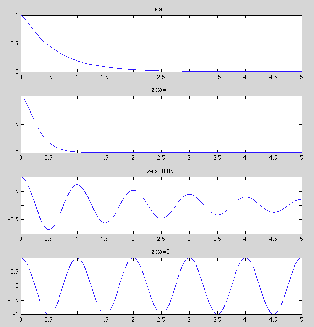
The homogeneous responses of these four cases are plotted below. Note that in all cases, $y(0)=y_0$ and $\dot{y}(0)=0$.