Gaussian mixture model

In K-means clustering, each sample point ${\bf x}$ is assigned to one of the $K$ clusters if it has the minimum Euclidean distance to the mean of the cluster. But here the distribution of the data samples in the cluster represented by the covariance is not taken into consideration.

This issue can be addressed by the method of Gaussian mixture model (GMM) based on the assumption that each of the $K$ clusters $\{C_1,\cdots,C_K\}$ in the given dataset can be modeled by a Gaussian distribution ${\cal N}({\bf x}; {\bf m}_k,{\bf\Sigma}_k),\;(k=1,\cdots,K)$ in terms of both the mean vector ${\bf m}_k$ and covariance matrix ${\bf\Sigma}_k$. The overall distribution of the entire dataset ${\bf X}=[{\bf x}_1,\cdots,{\bf x}_N]$ is the weighted sum of the $K$ Gaussian distributions:

$$p({\bf x})=\sum_{k=1}^K P_k {\cal N}({\bf x}; {\bf m}_k,{\bf\Sigm... ...{1}{2}({\bf x}-{\bf m}_k)^T {\bf\Sigma}_k^{-1}({\bf x}-{\bf m}_k)\right)\right]$$ (209)

where $P_k$ is the weight for the kth Gaussian ${\cal N}({\bf x}; {\bf m}_k,{\bf\Sigma}_k)$, satisfying

$$\int_{-\infty}^\infty p({\bf x})\,d{\bf x} =\sum_{k=1}^K P_k \int... ...infty {\cal N}({\bf x}; {\bf m}_k,{\bf\Sigma}_k)\,d{\bf x} =\sum_{k=1}^K P_k =1$$ (210)

The GMM clustering is carried out by the method of expectation maximization (EM), by which all model parameters denoted by $\theta =\{P_k,{\bf m}_k,{\bf\Sigma}_k,\;(k=1,\cdots,K)\}$ are estimated based on the given dataset, and then each sample in the dataset is assigned to one of the clusters.

We note that the GMM model in Eq. (209) is actually the same as Eq. (11) in the naive Bayes classification. These two methods are similar in the sense that each cluster or classe $C_k$ is modeled by a Gaussian ${\cal N}({\bf x},{\bf m}_k,{\bf\Sigma}_k)$, weighted by $P_k$, and the model parameters ${\bf m}_k$ and ${\bf\Sigma}_k$, as well as $P_k$, are to be estimated based on the given dataset. However, the two methods are different in that the dataset ${\bf X}$ in the supervised naive Bayes method is labeled by ${\bf y}$, while in GMM such a labeling vector is not available. Instead, here we will introduce a latent or hidden variable ${\bf z}=[z_1,\cdots,z_K]^T$ as the cluster labeling of the samples in the given dataset ${\bf X}$. This latent variable ${\bf z}$ is binary vector, of which each component is a binary random variable $z_k\in\{0,\,1\}$. Only one of these $K$ components is 1, e.g., $z_k=1$, indicating a sample ${\bf x}$ in the dataset belongs to the kth cluster $C_k$, while all others are 0, i.e., these $K$ binary variables add up to 1, $\sum_{k=1}^K z_k=1$.

We further introduce the following probabilities for each of the $K$ clusters $C_k\;\;(k=1,\cdots,K)$:

• The prior probability for any unobserved data sample ${\bf x}\in{\bf X}$ in the dataset to belong to $C_k$, represented by $z_k=1$:

  $$P(z_k=1)=P_k\;\;\;\;\;(k=1,\cdots,K)\;\;\;\;\; \;\;\;\;\; \sum_{k=1}^K P_k=1$$ (211)

  These $K$ prior probabilities add up to 1, i.e, the $K$ events $z_k=1\;(k=1,\cdots,K)$ are mutually exclusive and complementary, as any sample ${\bf x}$ belongs to one and only one of the $K$ clusters.

• The probability distribution of all samples in $C_k$, assumed to be a Gaussian:

  $$p({\bf x}\vert z_k=1,\theta)={\cal N}({\bf x};{\bf m}_k,{\bf\Sigma}_k)$$ (212)

• The joint distribution of any ${\bf x}$ and $z_k=1$:

  $$p({\bf x},z_k=1\vert\theta)=p({\bf x}\vert z_k=1,\theta)\;P(z_k=1) =P_k {\cal N}({\bf x};{\bf m}_k,{\bf\Sigma}_k)$$ (213)

Marginalizing this joint probability over the latent variable $z_k$, we get the Gaussian mixture model, the distribution $p({\bf x})$ of any sample ${\bf x}$ regardless to which cluster it belongs:

$$p({\bf x}\vert\theta)=\sum_{k=1}^K p({\bf x},z_k=1\vert\theta) =\... ...,\theta)\;P(z_k=1) =\sum_{k=1}^K P_k {\cal N}({\bf x}; {\bf m}_k,{\bf\Sigma}_k)$$ (214)

Note that Eqs. (211) through (214) are the same as Eqs. (8) through (11) in the naive Bayes classifier, respectively.

All such probabilities defined for $z_k=1$ can be generalized to ${\bf z}=[z_1,\cdots,z_K]^T$ for all $K$ clusters:

$$p({\bf z}\vert{\bf\theta}) = \prod_{k=1}^K P_k^{z_k}$$ (215)

$$p({\bf x}\vert{\bf z},{\bf\theta}) = \prod_{k=1}^K {\cal N}({\bf x},{\bf m}_k,{\bf\Sigma}_k)^{z_k}$$ (216)

$$p({\bf x},{\bf z}\vert{\bf\theta}) = p({\bf z})\;p({\bf x}\vert{\bf z},\theta) =\prod_{k=1}^K \left(P_k {\cal N}({\bf x},{\bf m}_k,{\bf\Sigma}_k)\right)^{z_k}$$ (217)

Given the dataset ${\bf X}=[{\bf x}_1,\cdots,{\bf x}_N]$ containing $N$ i.i.d. samples, we introduce $N$ corresponding latent variables in ${\bf Z}=[{\bf z}_1,\cdots,{\bf z}_N]$, of which the nth column ${\bf z}_n=[z_{n1},\cdots,z_{nK}]^T$ is the labeling vector of ${\bf x}_n$, i.e., ${\bf x}_n$ belongs to $C_k$ if $z_{nk}=1$ (while $z_{nl}=0$ for all $l\ne k$). Note that here ${\bf Z}=[{\bf z}_1,\cdots,{\bf z}_N]$ is defined in the same way as ${\bf Y}=[{\bf y}_1,\cdots,{\bf y}_N]$ in softmax regression, both as the labeling of ${\bf X}$, with the only difference that ${\bf Y}$ is provided in the training data available for a supervised method, but here ${\bf Z}$ is a latent variable not part of the data provided for unsupervised clustering. Now we have

$$p({\bf x}_n,{\bf z}_n\vert\theta)=\prod_{k=1}^K \left(P_k {\cal N... ...m}_k,{\bf\Sigma}_k)\right)^{z_{nk}}, \;\;\;\;\;\;\;\;\;\;\;\;\;\;(n=1,\cdots,N)$$ (218)

The likelihood function of the GMM model parameters ${\bf\theta}$ to be estimated can be expressed as:

$$L(\theta\vert{\bf X},{\bf Z}) = p({\bf X},{\bf Z}\vert\theta) =p\left([{\bf x}_1,\cdots,{\bf x}_N... ...}_1,\cdots,{\bf z}_N]\bigg\vert{\bf m}_k,{\bf\Sigma}_k,P_k(k=1,\cdots,K)\right)$$

$$= \prod_{n=1}^N p({\bf x}_n,{\bf z}_n\vert\theta) =\prod_{n=1}^N \prod_{k=1}^K \left(P_k{\cal N}({\bf x}_n,{\bf m}_k,{\bf\Sigma}_k)\right)^{z_{nk}}$$ (219)

and the log likelihood is:

$$l({\bf\theta}\vert{\bf X},{\bf Z})= \log L(\theta\vert{\bf X},{\bf Z}) = \log p({\bf X},{\bf Z}\vert\theta) =\log \left[ \prod_{n=1}^N \pr... ...}^K \left(P_k{\cal N}({\bf x}_n,{\bf m}_k,{\bf\Sigma}_k)\right)^{z_{nk}}\right]$$

$$= \sum_{n=1}^N \sum_{k=1}^K z_{nk} \left[\log P_k+\log {\cal N}({\bf x}_n,{\bf m}_k,{\bf\Sigma}_k)\right]$$ (220)

Similar to the method of maximum likelihodd estimation (MLE) which finds the model parameters in ${\bf\theta}$ as those that maximize the likelihood function $L({\bf\theta})$ or its log function $\log\;L({\bf\theta})$, here we find the model parameters in $\theta =\{P_k,{\bf m}_k,{\bf\Sigma}_k,\;(k=1,\cdots,K)\}$ as those that maximize the expectation of the log likelihood function above with respect to the latent variables in ${\bf Z}$ in the following two iterative steps of the EM method:

• E-step: Find the expectation of the log likelihood function.

  We first find the posterior probability for an observed ${\bf x}_n$ to belong to cluster $C_k$, indicated by $z_{nk}=1$ (and $z_{nl}=0$ for all $l\ne k$):
  

  $$P_{nk} = P(z_{nk}=1\vert{\bf x}_n,\theta) =\frac{p({\bf x}_n,z_{nk}=1\vert... ...k{\bf\Sigma}_k)} {\sum_{l=1}^K P_l\,{\cal N}({\bf x}_n;{\bf m}_l{\bf\Sigma}_l)}$$

  $$(n=1,\cdots,N;\;k=1,\cdots,K)$$ (221)

  
  As ${\bf x}_n$ has to belong to one of the $K$ clusters, these $K$ posterior probabilities add up to 1, same ss the prior probabilities $P(z_k=1)=P_k$:

  $$\sum_{k=1}^K P(z_k=1)=\sum_{k=1}^K P_k=1, \;\;\;\;\;\;\;\;\;\;\;\;\;\; \sum_{k=1}^K P(z_{nk}=1\vert{\bf x}_n,\theta)=\sum_{k=1}^K P_{nk}=1$$ (222)

  This posterior probability $P_{nk}=p(z_{nk}=1\vert{\bf x}_n,\theta)$ can be considered as the responsibility cluster $C_k$ takes for ${\bf x}_n$. Once we have available all parameters on the right-hand side of Eq. (221) for $P_{nk}$, it is used to assign each sample ${\bf x}_n$ to a cluster $C_k$ with the maximun responsibility $P_{nk}=\max_l P_{nl}$.

  We note that the definition of $P_{nk}$ is similar to the softmax function $s_{nk}$ with the only difference that here the weighted Gaussian function are used instead of the softmax function used in softmax regression.

  We also note that the posterior probability $P_{nk}$ defined above represents a soft decision, in the sense that it is possible for any ${\bf x}_n$ to belong to any $C_k$ with probability $0<P_{nk}<1$ for all $k=1,\cdots,K$, instead of a hard decision, in the sense that ${\bf x}_n$ belongs to only one specific $C_k$ with $P_{nk}=1$, while $P_{nl}=0$ for all $l\ne k$, as in K-means clustering.

  We can now find the expectation of the log likelihood with respect to the latent variables in ${\bf Z}$:
  

  $$E_Z\left( \log L(\theta\vert{\bf X},{\bf Z}) \right) = E_Z\left[\sum_{n=1}^N \sum_{k=1}^K z_{nk} \left[\log P_k+\log {\cal N}({\bf x}_n,{\bf m}_k,{\bf\Sigma}_k)\right]\right]$$

  $$= \sum_{n=1}^N \sum_{k=1}^K E_Z(z_{nk}) \left[\log P_k+\log {\cal N}({\bf x}_n,{\bf m}_k,{\bf\Sigma}_k)\right]$$

  $$= \sum_{n=1}^N \sum_{k=1}^K P_{nk} \left[\log P_k+\log {\cal N}({\bf x}_n,{\bf m}_k,{\bf\Sigma}_k)\right]$$ (223)

  
  The last equality is due to the following fact:

  $$E_z(z_{nk})=1\;P(z_{nk}=1\vert{\bf x}_n)+0\;P(z_{nk}=0\vert{\bf x}_n) =P(z_{nk}=1\vert{\bf x}_n)=P_{nk}$$ (224)

• M-step: Find the optimal model parameters that maximize the expectation of the log likelihood.

  We first set to zero the derivatives of the expectation of the log likelihood with respect to each of the parameters in ${\bf\theta}=\{P_k,\;{\bf m}_k,\;{\bf\Sigma}_k,\;(k=1,\cdots,K)\}$, and then solve the resulting equations to get the optimal parameters.

  • Find $P_k$:

    As all $K$ of $P_k$'s need to satisfy the constraint $\sum_{k=1}^K P_k=1$, we first construct the Lagrangian function composed of an extra Lagrange multiplier term for the constraint as well as the log likelihood as the objective function:

    $$L(\theta,\,\lambda) =\sum_{n=1}^N \sum_{k=1}^K P_{nk} \left[\log ... ...bf x}_n,{\bf m}_k,{\bf\Sigma}_k)\right] +\lambda\left(\sum_{k=1}^K P_k-1\right)$$ (225)

    and set it derivative with respect to $P_k$ to zero:
    

    $$\frac{\partial}{\partial P_k} L(\theta,\,\lambda) = \frac{\partial}{\partial P_k} \left[ \sum_{n=1}^N \sum_{k=1}^K P_... ...{\bf m}_k,{\bf\Sigma}_k)\right] +\lambda\left(\sum_{k=1}^K P_k-1\right) \right]$$

    $$= \sum_{n=1}^N P_{nk}\frac{1}{P_k}+\lambda=0$$ (226)

    
    Multiplying both sides by $P_k$, we get

    $$\sum_{n=1}^N P_{nk}+P_k \lambda=N_k+P_k\lambda=0$$ (227)

    where we have defined

    $$N_k=\sum_{n=1}^N P_{nk}$$ (228)

    that satisfies

    $$\sum_{k=1}^K N_k=\sum_{k=1}^K\left(\sum_{n=1}^N P_{nk}\right) =\sum_{n=1}^N\left(\sum_{k=1}^K P_{nk}\right)=\sum_{n=1}^N 1=N$$ (229)

    Summing Eq. (227) over all $k=1,\cdots,K$, we get

    $$\sum_{k=1}^K\left(N_k+P_k \lambda\right) =\sum_{k=1}^K N_k+\lambda\left(\sum_{k=1}^K P_k\right) =N+\lambda=0$$ (230)

    Substituting $\lambda=-N$ back into Eq. (227), we get the expression for the prior

    $$p(z_k=1)=P_k=\frac{N_k}{N}=\frac{1}{N}\sum_{n=1}^N P_{nk}$$ (231)

    This is actually the same as the prior $P_k$ in Eq. (8) in naive Bayes classification, but here $N_k$ defined in Eq. (228) is the sum of the probabilities for all $N$ data samples to belong to $C_k$, instead of the number of data samples in $C_k$ (unknown in this unsupervised case).

  • Find ${\bf m}_k$:

    
    

    $$\frac{\partial}{\partial{\bf m}_k} E_Z(\log L(\theta\vert{\bf X},{\bf Z})) = \frac{\partial}{\partial{\bf m}_k} \left[\sum_{n=1}^N \sum_{l=1}^... ...} \left[\log P_l+\log {\cal N}({\bf x}_n,{\bf m}_l,{\bf\Sigma}_l)\right]\right]$$

    $$= \sum_{n=1}^N P_{nk}\frac{\partial}{\partial{\bf m}_k} \log {\cal N}({\bf x}_n,{\bf m}_k,{\bf\Sigma}_k)$$

    $$\stackrel{*}{=} \sum_{n=1}^N P_{nk}\frac{\partial}{\partial{\bf m}_k} \left[-\frac{1}{2}({\bf x}_n-{\bf m}_k)^T{\bf\Sigma}_k^{-1}({\bf x}_n-{\bf m}_k)\right]$$

    $$= \frac{1}{2}\sum_{n=1}^N P_{nk}{\bf\Sigma}_k^{-1}({\bf x}_n-{\bf m}_k)={\bf0}$$ (232)

    
    Note that here $\stackrel{*}{=}$ indicates that we have neglected the scaling coefficient $(2\pi)^{-d/2}\,\vert{\bf\Sigma}_k\vert^{-1/2}$ of the Gaussian, which is independent of ${\bf m}_k$. Multiplying $2{\bf\Sigma}_k$ on both sides, we get

    $$\sum_{n=1}^N P_{nk}({\bf x}_n-{\bf m}_k) =\sum_{n=1}^N P_{nk}{\bf... ...-\sum_{n=1}^N P_{nk}{\bf m}_k =\sum_{n=1}^N P_{nk}{\bf x}_n-N_k{\bf m}_k={\bf0}$$ (233)

    Solving for ${\bf m}_k$ we get

    $${\bf m}_k=\frac{1}{N_k}\sum_{n=1}^N P_{nk}{\bf x}_n$$ (234)

  • Find ${\bf\Sigma}_k$:

    
    

    $$\frac{\partial}{\partial{\bf\Sigma}_k} E_Z(\log L(\theta\vert{\bf X},{\bf Z})) = \frac{\partial}{\partial{\bf\Sigma}_k} \left[\sum_{n=1}^N \sum_{l... ...} \left[\log P_l+\log {\cal N}({\bf x}_n,{\bf m}_l,{\bf\Sigma}_l)\right]\right]$$

    $$= \sum_{n=1}^N P_{nk}\frac{\partial}{\partial{\bf\Sigma}_k} \log {\cal N}({\bf x}_n,{\bf m}_k,{\bf\Sigma}_k)$$

    $$= -\frac{1}{2}\sum_{n=1}^N P_{nk} \left[\frac{\partial}{\partial{\b... ...\Sigma}_k}({\bf x}_n-{\bf m}_k)^T{\bf\Sigma}_k^{-1}({\bf x}_n-{\bf m}_k)\right]$$

    $$= -\frac{1}{2}\sum_{n=1}^N P_{nk} \left[{\bf\Sigma}_k^{-1}-{\bf\Sig... ...1} ({\bf x}_n-{\bf m}_k)({\bf x}_n-{\bf m}_k)^T{\bf\Sigma}_k^{-1}\right]={\bf0}$$ (235)

    
    Here we have used the following facts (for more details see Matrix Cookbook):

    $$\frac{d}{d{\bf A}}\log\vert{\bf A}\vert=({\bf A}^{-1})^T, \;\;\;\... ...^T{\bf A}^{-1}{\bf b}\right) =-({\bf A}^{-1})^T{\bf a}{\bf b}^T({\bf A}^{-1})^T$$ (236)

    Pre and post multiplying ${\bf\Sigma}_k$ on both sides of the equation above we get

    $$\sum_{n=1}^N P_{nk}\left({\bf\Sigma}_k-({\bf x}_n-{\bf m}_k)({\bf x}_n-{\bf m}_k)^T\right)={\bf0}$$ (237)

    Solving for ${\bf\Sigma}_k$, we get

    $${\bf\Sigma}_k=\frac{1}{N_k}\sum_{n=1}^N P_{nk}({\bf x}_n-{\bf m}_k)({\bf x}_n-{\bf m}_k)^T$$ (238)

We note that all model parameters in ${\bf\theta}=\{P_k,{\bf m}_k,{\bf\Sigma}_k,(k=1,\cdots,K)\}$ found respectively in Eqs. (231), (234), and (238) in the M-step depend on $P_{nk}$ in Eq. (221) in the E-step, which in turn is a function of these parameters, i.e., the E-step and M-step need to be carried out in an alternative and iterative fashion from some initial values of the parameters until convergence.

In summary, here is the EM clustering algorithm based on Gaussian mixture model:

1. Initialize means ${\bf m}_k$, covariance ${\bf\Sigma}_k$ and coefficient $P_k$.

2. The E-step:

   Find the responsibility $P_{nk}$ for all $N$ data points and all $K$ clusters and then $N_k$:

   $$P_{nk}=P(r_k=1\vert{\bf x}_n) =\frac{P_k\,{\cal N}({\bf x}_n;{\bf... ...l N}({\bf x}_n;{\bf m}_l,{\bf\Sigma}_l)}, \;\;\;\;\;\;\;N_k=\sum_{n=1}^N P_{nk}$$ (239)

3. The M-step:

   Recalculate the parameters that maximize the likelihood function:
   

   $$P_k = \frac{N_k}{N}$$

   $${\bf m}_k = \frac{1}{N_k} \sum_{n=1}^N P_{nk}{\bf x}_n$$

   $${\bf\Sigma}_k = \frac{1}{N_k}\sum_{n=1}^N P_{nk}({\bf x}_n-{\bf m}_k)({\bf x}_n-{\bf m}_k)^T$$ (240)

   
   

4. If the parameters or the log likelihood function have not converged, go back to step 2. Otherwise terminate the iteration. The probability for each sample ${\bf x}_n$ to belong to cluster $C_l$ is $p_{nl}=P(z_{nl}=1\vert{\bf x}_n,\theta)$, and it is therefore assigned to $C_k$ if $P_{nk}=\max_l p_{nl}$.

We can show that the K-means algorithm is actually a special case of the EM algorithm, when all covariance matrices are the same ${\bf\Sigma}_k=\varepsilon{\bf I}$, where $\varepsilon$ is a scaling factor which appraoches to zero. In this case we have:

$$p({\bf x}\vert z_k=1,\theta)={\cal N}({\bf x}\vert{\bf m}_k,\vare... ...\exp\left(-\frac{1}{2\varepsilon}\vert\vert{\bf x}-{\bf m}_k\vert\vert^2\right)$$ (241)

and the probability for any ${\bf x}_n\in{\bf X}$ to belong to cluster $C_k$ is:

$$P_{nk}=P(z_k=1\vert{\bf x}_n,\theta) =\frac{P_k{\cal N}({\bf x}_n... ...{\sum_{l=1}^K P_l\exp(-\vert\vert{\bf x}_n-{\bf m}_l\vert\vert^2/2\varepsilon)}$$ (242)

When $\varepsilon\rightarrow 0$, all terms in the denominator approach to zero, but the one with minimum $\vert\vert{\bf x}-{\bf m}_k\vert\vert$ approaches to zero most slowly, and becomes the dominant term of the denominator. If the numerator happens to be this term as well, then $P_{nk}=1$, otherwise the numerator approaches zero and $P_{nk}=0$. Now $P_{nk}$ defined above becomes:

$$\lim\limits_{\varepsilon\rightarrow 0} P_{nk}=\lim\limits_{\varep... ...t\vert{\bf x}_n-{\bf m_l}\vert$}\vert\\ 0 & \mbox{otherwise}\end{array}\right.$$ (243)

Now the posterior probability $0<P_{nk}<1$ defined in Eq. (221) for a soft decision becomes a binary value $P_{nk}\in\{0,\;1\}$ for a hard binary decision to assign ${\bf x}_n$ to $C_k$ with the smallest distance. Also $N_k=\sum_{n=1}^N P_{nk}$ defined in Eq. (228) as the sum of the posterior probabilities for all $N$ data points to belong to $C_k$ becomes $N_k$ as the number of data samples assigned only to $C_k$. In other words, now the probabilistic EM method based on both ${\bf m}$ and ${\bf\Sigma}$ becomes the deterministic K-means method based on ${\bf m}$ only.

We can also make a comparison between the GMM method for unsupervised clustering and the softmax regression for supervised classification. First, the latent variables ${\bf Z}=[{\bf z}_1,\cdots,{\bf z}_N]$ in GMM play a similar role as the labeling ${\bf Y}=[{\bf y}_1,\cdots,{\bf y}_N]$ in softmax regression for multi-class classificatioin. However, the difference is that ${\bf Y}$ is explicitely given in the training set for a supervised classification, while ${\bf Z}$ is hidden for an unsupervised cllustering analysis. Second, we note that the probability $P_{nk}=p(z_{nk}=1\vert{\bf x}_n,\theta)$ given in Eq. (221) is similar to the softmax function $\phi_{nk}=P(y'=k\vert{\bf x}_n)$ in the softmax method in terms of their form, with the only difference that the Gaussian function is used for GMM while the exponential function is used for solfmax.

Examples

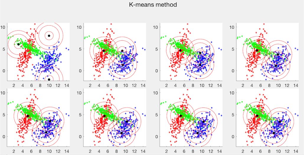
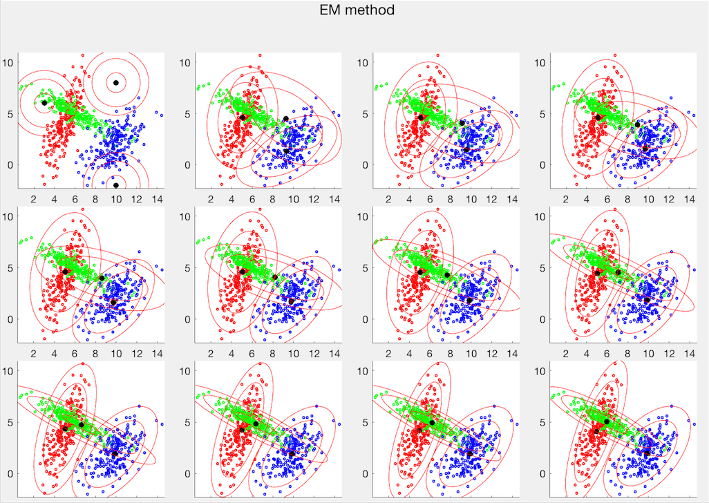
The same dataset is used to test both the K-means and EM clustering methods. The first panel shows 10 iterations of the K-means method, while the second panel shows 16 iterations of the EM method. In both cases, the iteration converges to the last plot. Comparing the two clustering results, we see that the K-means method cannot separate the red and green data points from two different clusters, both normally distributed with similar means but very different covariance matrices, while the blue data points all in the same cluster are separated into two clusters. But the EM method based on the Gaussian mixture model can correctly identified all three clusters.

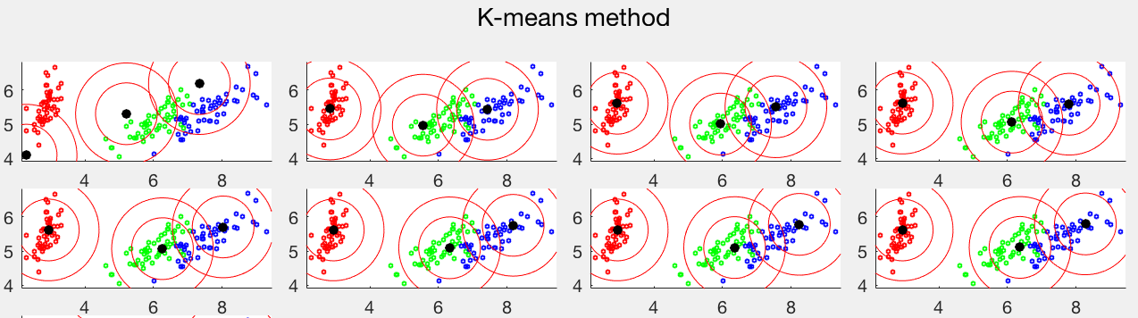
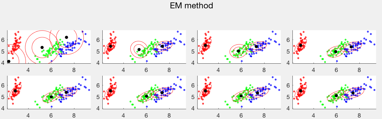
The two clustering methods are also applied to the Iris dataset, which has three classes each of 50 4-dimensional sample vectors. The PCA method is used to visualize the first two principal compnents, as shown below. Also, as can be seen from their c onfussion matrices, the error rate of the K-means method is 18/150, while that of the EM method is 5/150.

$$\begin{tabular}{r\vert r\vert r} \multicolumn{3}{c}{K-means}\\ \h... ...e 0 & 0 & 50\\ \hline45 & 5 & 0\\ \hline0 & 50 & 0\\ \hline\hline \end{tabular}$$ (244)