Mixture of Bernoulli

If the data are binary, i.e., each data point $x$ is treated as a discrete random variable that takes either of two binary values such as $1$ and 0 with probabilities $\mu$ and $1-\mu$, then the assumption of Gaussian distribution of the dataset is no longer valid and the Gaussian mixture model is not suitable. In this case, the probability mass function (pmf) of the Bernoulli distribution can be used instead:

$${\cal B}(x\vert\mu)=\mu^x(1-\mu)^{1-x}=\left\{\begin{array}{cl} \mu & \mbox{if $x=1$} \\ 1-\mu & \mbox{if $x=0$} \end{array}\right.$$ (245)

The mean and variance of $x$ are

$$E(x) = 1\;P(x=1)+0\;P(x=0)=1\;\mu+0\;(1-\mu)=\mu$$ (246)

$$Var(x) = E[(x-E(x))^2]=E(x^2)-E(x)^2$$

$$= 1^2\;P(x=1)+0^2\;P(x=0)-\mu^2=\mu-\mu^2=\mu(1-\mu)$$ (247)

A set of $d$ independent binary variables can be represented as a random vector ${\bf x}=[x_1,\cdots,x_d]^T$ with mean vector and covariance matrix as shown below:

$$E({\bf x}) = {\bf m}=[\mu_1,\cdots,\mu_N]^T$$ (248)

$$Cov({\bf x}) = {\bf\Sigma}=diag( \mu_i(1-\mu_i) ) =\left[ \begin{array}{ccc} \mu_1(1-\mu_1) & & 0 \\ & \ddots & \\ 0 & & \mu_d(1-\mu_d)\end{array}\right]$$ (249)

Note that the covariance matrix ${\bf\Sigma}$ is solely determined by the means $\{\mu_1,\cdots,\mu_N\}$.

Now we can get the pmf of the a binary random vector ${\bf x}$:

$${\cal B}({\bf x}\vert{\bf m})=\prod_{i=1}^d {\cal B}(x_i\vert\mu_i) =\prod_{i=1}^d \mu_i^{x_i}(1-\mu_i)^{1-x_i}$$ (250)

and the log pmf:

$$\log {\cal B}({\bf x}\vert{\bf m}) =\log\left(\prod_{i=1}^d {\cal... ...ert\mu_i)\right) =\sum_{i=1}^d \left[ x_i\log\mu_i+(1-x_i)\log(1-\mu_i) \right]$$ (251)

Similar to the Gaussian mixture model, the Bernoulli mixture model of $K$ multivariate Bernoulli distributions is defined as:

$$p({\bf x}\vert{\bf m}_k,P_k,(k=1,\cdots,K))=p({\bf x}\vert{\bf\th... ...},{\bf m}_k) =\sum_{k=1}^K P_k \prod_{i=1}^d \mu_{ki}^{x_i}(1-\mu_{ki})^{1-x_i}$$ (252)

where ${\bf\theta}=\{{\bf m}_k,P_k,(k=1,\cdots,K)\}$ denotes all parameters of the mixture model to be estimated based on the given dataset, and ${\bf m}_k=E_k({\bf x})$ respect to ${\cal B}({\bf x}\vert{\bf m}_k)$. The mean of this mixture model is

$${\bf m}=E({\bf x})=\sum_{k=1}^KP_k E_k({\bf x})=\sum_{k=1}^K P_k{\bf m}_k$$ (253)

Also similar to the Gaussian mixture model, we introduce a set of $K$ latent binary random variables ${\bf z}=[z_1,\cdots,z_K]^T$ with binary conponents $z_k\in\{0,\;1\}$ and $\sum_{k=1}^K z_k=1$, and get the prior probability of ${\bf z}$, the conditional probability of ${\bf x}$ given ${\bf z}$, and the joint probability of ${\bf x}$ and ${\bf z}$ as the following

$$p({\bf z}\vert{\bf\theta}) = \prod_{k=1}^K P_k^{z_k}$$ (254)

$$p({\bf x}\vert{\bf z},{\bf\theta}) = \prod_{k=1}^K {\cal B}({\bf x},{\bf m}_k)^{z_k}$$ (255)

$$p({\bf x},{\bf z}\vert{\bf\theta}) = p({\bf z}\vert{\bf\theta})\;p({\bf x}\vert{\bf z},{\bf\theta}) =\prod_{k=1}^K \left(P_k\;{\cal B}({\bf x},{\bf m}_k)\right)^{z_k}$$ (256)

Given the dataset ${\bf X}=[{\bf x}_1,\cdots,{\bf x}_N]$ containing $N$ i.i.d. samples, we introduce the corresponding latent variables in ${\bf Z}=[{\bf z}_1,\cdots,{\bf z}_N]$, of which each ${\bf z}_n=[z_{n1},\cdots,z_{nK}]^T$ is for the labeling of ${\bf x}_n$. Then we can find the likelihood function of the Bernoulli mixture model parameters ${\bf\theta}=\{P_k,{\bf m}_k,\;(k=1,\cdots,K)\}$:

$$L({\bf\theta}\vert{\bf X},{\bf Z})=p({\bf X},{\bf Z}\vert\theta) = p([{\bf x}_1,\cdots,{\bf x}_N],[{\bf z}_1,\cdots,{\bf z}_N] \vert{\bf m}_k,P_k(k=1,\cdots,K))$$

$$= \prod_{n=1}^N p({\bf x}_n,{\bf z}_n\vert{\bf\theta}) =\prod_{n=1}^N \prod_{k=1}^K \left(P_k{\cal B}({\bf x}_n,{\bf m}_k)\right)^{z_{nk}}$$ (257)

and the log likelihood function:

$$\log\;L({\bf\theta}\vert{\bf X},{\bf Z}) = \log p({\bf X},{\bf Z}\vert\theta) =\log\prod_{n=1}^N \prod_{k=1}^K \left(P_k{\cal B}({\bf x}_n,{\bf m}_k)\right)^{z_{nk}}$$

$$= \sum_{n=1}^N \sum_{k=1}^K {z_{nk}} \left[ \log P_k +\log {\cal B}({\bf x}_n,{\bf m}_k)\right]$$ (258)

Based on the same EM method used in Gaussian mixture model, we can find the opptimal parameters that maximize the expectation of the log likelihood function in the following two steps:

• E-step: Find the expectation of the likelihood function.

  We first find the posterior probability for any sample ${\bf x}_n$ to belong to cluster $C_k$, denoted by $P_{nk}$:
  

  $$P_{nk} = P(z_{nk}=1\vert{\bf x}_n,{\bf\theta}) =\frac{p({\bf x}_n,z_{nk}=1... ...\cal B}({\bf x}_n;{\bf m}_k)} {\sum_{l=1}^K P_l\,{\cal B}({\bf x}_n;{\bf m}_l)}$$

  $$(n=1,\cdots,N;\;\;k=1,\cdots,K)$$ (259)

  
  which is the expectation of $z_{nk}$:

  $$E(z_{nk})=1\;P(z_{nk}=1\vert{\bf x}_n)+0\;P(z_{nk}=0\vert{\bf x}_n) =P(z_{nk}=1\vert{\bf x}_n)=P_{nk}$$ (260)

  Now we can find the expectation of the log likelihood with respect to the latent variables in ${\bf Z}$:
  

  $$E_z \left(\log L({\bf\theta}\vert{\bf X},{\bf Z})\right) = E_z\;\sum_{n=1}^N \sum_{k=1}^K z_{nk}\left[\log P_k +\log {\cal B}({\bf x}_n,{\bf m}_k)\right]$$

  $$= \sum_{n=1}^N \sum_{k=1}^K E(z_{nk}) \left[\log P_k +\log \prod_{i=1}^d \mu_{ki}^{x_{ni}} (1-\mu_{ki})^{1-x_{ni}} \right]$$

  $$= \sum_{n=1}^N \sum_{k=1}^K P_{nk} \left[\log P_k +\sum_{i=1}^d \left[ x_{ni}\log\mu_{ki}+(1-x_{ni})\log(1-\mu_{ki}) \right]\right]$$ (261)

  
  

• M-step: Find the optimal model parameters that maximize the expectation of the log likelihood function.

  We first set to zero the derivatives of the expectation of the log likelihood with respect to each of the parameters in ${\bf\theta}=\{P_k,\;{\bf m}_k\;(k=1,\cdots,K)\}$, and then solve the resulting equations to get the optimal parameters.

  • Find $P_k$: same as in the case of the GMM model:

    $$P_k=\frac{N_k}{N}=\frac{1}{N}\sum_{n=1}^N P_{nk}$$ (262)

  • Find ${\bf m}_k$:
    

    $$\frac{\partial}{\partial{\bf m}_k} E_{\bf Z}\left( \log p({\bf X},{\bf Z}\vert\theta) \right)$$

    $$= \frac{\partial}{\partial{\bf m}_k} \sum_{n=1}^N \sum_{k=1}^K P_{n... ...sum_{i=1}^d \left[ x_{ni}\log\mu_{ki}+(1-x_{ni})\log(1-\mu_{ki}) \right]\right]$$

    $$= \sum_{n=1}^N P_{nk} \frac{\partial}{\partial{\bf m}_k} \sum_{i=1}^d\left[ x_{ni}\log\mu_{ki}+(1-x_{ni})\log(1-\mu_{ki}) \right]={\bf0}$$ (263)

    
    The ith component of the equation is
    

    $$\sum_{n=1}^N P_{nk}\frac{d}{d\mu_{ki}} \left[ x_{ni}\log \mu_{ki}+(1-x_{ni})\log(1-\mu_{ki})\right]$$

    $$= \sum_{n=1}^N P_{nk}\left(\frac{x_{ni}}{\mu_{ki}}-\frac{1-x_{ni}}{1-\mu_{ki}}\right)=0$$ (264)

    
    i.e.,

    $$(1-\mu_{ki})\sum_{n=1}^N P_{nk} x_{ni}=\mu_{ki}\sum_{n=1}^N P_{nk}(1-x_{ni}) =\mu_{ki}N_k-\mu_{ki} \sum_{n=1}^N P_{nk}x_{ni}$$ (265)

    Solving for $\mu_{ki}$ we get

    $$\mu_{ki}=\frac{1}{N_k}\sum_{n=1}^N P_{nk}x_{ni}\;\;\;\;\;\;(i=1,\cdots,d)$$ (266)

    or, in vector form,

    $${\bf m}_k=\frac{1}{N_k}\sum_{n=1}^N P_{nk}{\bf x}_n$$ (267)

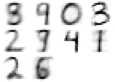
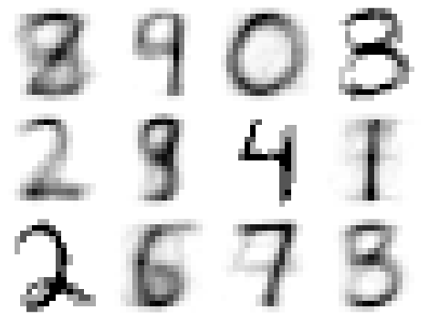
  Example:

  Clustering results of hand-written digits with $K=10$ and $K=12$. The mean vectors ${\bf m}_k$ of each of the $K$ clusters are visualized as shown: