Next: Gaussian mixture model Up: Clustering Analysis Previous: Clustering Analysis
As suggested by the name of K-means clustering, in this method a set
of  mean vectors
 are used to represent
the clusters in the feature space, based on the assumption that there
exist a set of clusters in the dataset.
are used to represent
the clusters in the feature space, based on the assumption that there
exist a set of clusters in the dataset.
The K-means clustering algorithm can be formulated as an optimization problem to minimize an objective function
 |
(199) |
 |
(200) |
 is assigned to the kth cluster
  if its
distance to the mean
if its
distance to the mean  is minimum. To minimize the objective
function
is minimum. To minimize the objective
function  with respective to , we set its derivative with
respect to each to zero:
with respective to , we set its derivative with
respect to each to zero:
 |
(201) |
:
 |
(202) |
 is the number of all samples assigned to
cluster , and the summation is over all samples assigned to .
is the number of all samples assigned to
cluster , and the summation is over all samples assigned to .
As  depends on while in turn also depends
on , the steps above need to be carried out iteratively, starting
with randomly initialized mean vectors which are revised iteratively
until convergence. Here are steps of the process:
depends on while in turn also depends
on , the steps above need to be carried out iteratively, starting
with randomly initialized mean vectors which are revised iteratively
until convergence. Here are steps of the process:
clusters,
such as any samples of the dataset:
 ,
set iteration index to zero
,
set iteration index to zero  ;
;
 in the dataset to one
of the clusters according to its distance to the corresponding
mean vector:
in the dataset to one
of the clusters according to its distance to the corresponding
mean vector:
if then then |
(203) |
 denotes the kth cluster with mean vector
 in the lth iteration;
 so that the objective function given above, i.e., the sum of
the distances squared from all
so that the objective function given above, i.e., the sum of
the distances squared from all
 to
to
 is minimized:
 |
(204) |
 |
(205) |
 , go back to Step 2.
This method is simple and effective, but it has the main drawback
that the number of clusters needs to be estimated based on some
prior knowledge, and it stays fixed through out the clustering process,
even it may turn out later that the dataset may be better fit with
more or fewer clusters. One way to resolve this is to carry out the
algorithm multiple times with different , and then evaluate each
result based on the objective function , or some other separability
criteria, such as
 .
.
The Matlab code for the iteration loop of the algorithm is listed
below, where Mold and Mnew are respectively the mean
vectors before and after each modification. The iteration terminates
when the mean vectors no longer change.
    Mnew=X(:,randi(N,1,K));          % use any K random samples as initial means
    er=inf;
    while er>0                       % main iteration
        Mold=Mnew;
        Mnew=zeros(d,K);             % initialize new means
        Number=zeros(1,K);
        for i=1:N                    % for all N samples
            x=X(:,i);
            dmin=inf;
            for k=1:K                % for all K clusters
                d=norm(x-Mold(:,k));
                if d<dmin
                    dmin=d;  j=k;
                end
            end
            Number(j)=Number(j)+1;
            Mnew(:,j)=Mnew(:,j)+x;
        end
        for k=1:K
            if Number(k)>0
                Mnew(:,k)=Mnew(:,k)/Number(k);
            end
        end
        er=norm(Mnew-Mold);          % terminate if means no longer change
    end
Example 1
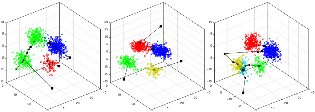
The K-means algorithm is applied to a simulated dataset in 3-D space with
 clusters. The results are shown in the figure below, where the three
panels show the results corresponding to
clusters. The results are shown in the figure below, where the three
panels show the results corresponding to  (left),
  (middle),
and
(middle),
and  (right). The initial positions of the means are marked
by the black squares, while their subsequent positions through out the
iteration are marked by smaller dots. The iteration terminates once the
means have moved to the centers of the clusters and no longer change
positions.
(right). The initial positions of the means are marked
by the black squares, while their subsequent positions through out the
iteration are marked by smaller dots. The iteration terminates once the
means have moved to the centers of the clusters and no longer change
positions.
The clustering results corresponding to
 can be evaluated
by the separability
, the intra-cluster
istance
can be evaluated
by the separability
, the intra-cluster
istance
 of the resulting clusters:
 |
(206) |
 inter-cluster (Bhattacharyya) distances (between any
two of the clusters):
inter-cluster (Bhattacharyya) distances (between any
two of the clusters):
 |
(207) |
 , the intra-cluster distance of the 2nd cluster is
significantly greater than the other two, indicating the cluster may contain
two smaller clusters. Also, when
, the intra-cluster distance of the 2nd cluster is
significantly greater than the other two, indicating the cluster may contain
two smaller clusters. Also, when  , the inter-cluster distance between
clusters 3 and 4 is significantly smaller than others, indicating the two
clusters are too close and can therefore be merged.
, the inter-cluster distance between
clusters 3 and 4 is significantly smaller than others, indicating the two
clusters are too close and can therefore be merged.
While the K-means method is simple and effective, it has the main shortcoming
that the number of clusters needs to be specified, although in practice it
is typically unknown a head of time. In this case, one could try different
values and compare the corresponding results in terms of the intra and inter
cluster distances, as well as the separabilities of the resulting clusters, as
shown in the example above. Moreover, if the intra-cluster distance of a cluster
is too large indicating it may contain more than one cluster (e.g.,  in
the example), it can be split; on the other hand, if the inter-cluster distance
between two clusters is too small (e.g.,
in
the example), it can be split; on the other hand, if the inter-cluster distance
between two clusters is too small (e.g.,  in the example), the two clusters
may belong to the same cluster and need to be merged. Following such merging
and/or splitting, a few more iterations can be carried out to make sure the
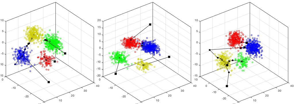
final clustering results are optimal. The figure below shows the clustering
results of the same dataset above but modified by merging and splliting. The
left pannel is for , but the second cluster (green) is split, while the
right pannel is for , when the 4th (yellow) and 5th (cyan) clusters are
merged.
in the example), the two clusters
may belong to the same cluster and need to be merged. Following such merging
and/or splitting, a few more iterations can be carried out to make sure the
final clustering results are optimal. The figure below shows the clustering
results of the same dataset above but modified by merging and splliting. The
left pannel is for , but the second cluster (green) is split, while the
right pannel is for , when the 4th (yellow) and 5th (cyan) clusters are
merged.
The idea of modifying the clustering results by merging and spliting leads to
the algorithm of Iterative Self-Organizing Data Analysis Technique (ISODATA),
which allows the number of clusters to be adjusted automatically during the
iteration by merging clusters close to each other and splitting clusters with
large intra-cluster distances. However, this algorithm is highly heuristic as
the various parameters such the threshold values for merging and splitting need
to be specified.
Example 2
The K-means clustering method is applied to the dataset of ten handwritten digits from 0 to 9 used previously. The clustering result is visualized based on the KLT that maps the data samples in the original 256-D space into the 3-D space spanned by the three eigenvectors corresponding to the three greatest eigenvalues of the covariance matrix of the dataset. The ground truth labelings are color coded as shown on the left, while the clustering result is shown on the right. We see that the clustering results match the original data reasonably well.
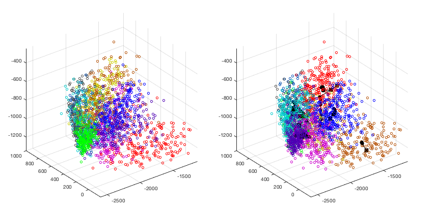
The clustering result is also shown in the confusion matrix, of which the columns and rows represent respectively the clusters based on the K-means clustering and the ground truth labeling (not used). In other words, the element in the ith row and jth column is the number of samples labeled to belong to the ith class but assigned to the jth cluster.
![$\displaystyle \left[ \begin{array}{rrrrrrrrrr}
1 & 0 & 25 & 165 & 27 & 2 & 3 & ...
...2 & 0 & 54 \\
4 & 2 & 0 & 1 & 0 & 28 & 119 & 1 & 64 & 5 \\
\end{array}\right]$](img777.svg) |
(208) |
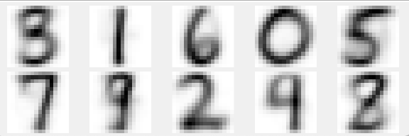
All samples are converted from 256-dimensional vector back to
 image form and the averages of the samples in each
of the ten cluster are shown in the figure below. We see that each
of the ten clusters clearly represents one distinct digit.
image form and the averages of the samples in each
of the ten cluster are shown in the figure below. We see that each
of the ten clusters clearly represents one distinct digit.