Naive Bayes Classification

The method of naive Bayes (NB) classification is a classical supervised classification algorithm, which is first trained by a training set of $N$ samples ${\bf X}=[{\bf x}_1,\cdots,{\bf x}_N]$ and their corresponding labelings ${\bf y}=[ y_1,\cdots,y_N]^T$, and then used to classify any unlabeled sample ${\bf x}$ into class $C_k$ with the maximumm posterior probability. As indicated by the name, naive Bayes classification is based on Bayes' theorem:

$$P(C_k\vert{\bf x})=\frac{p({\bf x},C_k)}{p({\bf x})} =\frac{p({\bf x}\vert C_k)P(C_k)}{p({\bf x})}$$ (7)

where

• $P(C_k)$ is the prior probability that any data sample belongs to class $C_k$ without observing its values, more briefly denoted by $P_k$, which can be estimated by

  $$P_k=\frac{N_k}{N}=\frac{N_k}{\sum_{l=1}^K N_l}, \;\;\;\;\;\;\;(k=1,\cdots,K)\;\;\;\;\;\; \;\;\;\;\; \sum_{k=1}^K P_k=1$$ (8)

  where $N_k$ is the number of data samples in the training set labeled to belong to class $C_k$. This estimation is based on the assumption that the training samples are evenly drawn from the entire population, and are therefore a fair representation of all $K$ classes.

• $p({\bf x}\vert C_k)=L(C_k\vert{\bf x})$ is the likelihood for any observed ${\bf x}$ to belong to class $C_k$, which is the conditional probability of ${\bf x}$ given that ${\bf x}\in C_k$, assumed to be a Gaussian in terms of the mean vector ${\bf m}_k$ and covariance matrix ${\bf\Sigma}_k$:

  $$p({\bf x}\vert C_k)=N({\bf x},{\bf m}_k,{\bf\Sigma}_k) =\frac{1}{... ...[-\frac{1}{2}({\bf x}-{\bf m}_k)^T{\bf\Sigma}_k^{-1} ({\bf x}-{\bf m}_k)\right]$$ (9)

  This assumption is based on the fact that the Gaussian distribution has the maximum entropy (uncertainty) among all probability density functions with the same covariance, i.e., it imposes the least amount of unsupported constraint on the model for the dataset.

• $p({\bf x},C_k)$ is the joint probability of ${\bf x}$ and $C_k$:

  $$p({\bf x},C_k)=p({\bf x}\vert C_k)P(C_k)=P(C_k\vert{\bf x})p({\bf x})$$ (10)

• $p({\bf x})$ is the distribution of any data sample in the dataset, independent of its classe identity, the weighted sum of all likelihood $p({\bf x}\vert C_k)$ for $k=1,\cdots,K$, i.e., the joint probability $p({\bf x},C_k)$ marginalized over all $K$ classes:

  $$p({\bf x})=\sum_{k=1}^K p({\bf x},C_k)=\sum_{k=1}^K P_k \,p({\bf ... ...1}{2}({\bf x}-{\bf m}_k)^T{\bf\Sigma}_k^{-1} ({\bf x}-{\bf m}_k)\right) \right]$$ (11)

• $P(C_k\vert{\bf x})$ is the posterior probability that a data sample ${\bf x}$ belongs to class $C_k$ based on the observed values in ${\bf x}=[x_1,\cdots,x_d]^T$.

Based on Bayes' theorem discussed above, the naive Bayes method classifies an unlabeled data sample ${\bf x}$ to class $C_k$ with the maximum posterior probability (maximum a posteriori (MAP)):

$$\;\;P(C_k\vert{\bf x})=\max_l\{ P(C_l\vert{\bf x}),\;(l=1,\cdots,K)\}, \;\;\;\; \;\;{\bf x}\in C_k$$ (12)

As $p({\bf x})$ is common to all $K$ classes (independent of $k$), it plays no role in the relative comparison among the $K$ classes, and can therefore be dropped, i.e., ${\bf x}$ is classified to $C_k$ with maximal $p({\bf x}\vert C_k)\,P_k$.

The naive Bayes classifier is an optimal classifier in the sense that the classification error is minimum. To illustrate this, consider an arbitrary boundary between two classes $C_1$ and $C_2$ that partitions the 1-D feature space into two regions $R_1$ and $R_2$, as shown below. The probability of a misclassification is the joint probability $P( {\bf x}\in C_i \cap {\bf x}\in R_j)$ for a sample ${\bf x}\in C_i$ but falling in $R_j$. The total probability of error due to misclassification can be expressed as:

$$P(error) = P(({\bf x}\in R_2) \cap ({\bf x}\in C_1)) +P(({\bf x}\in R_1) \cap ({\bf x}\in C_2))$$

$$= P({\bf x} \in R_2/C_1)\,P_1 +P({\bf x} \in R_1/C_2)\,P_2$$

$$= P_1 \int_{R_2}p({\bf x}/C_1)d{\bf x} +P_2\int_{R_1}p({\bf x}/C_2)d{\bf x}$$ (13)

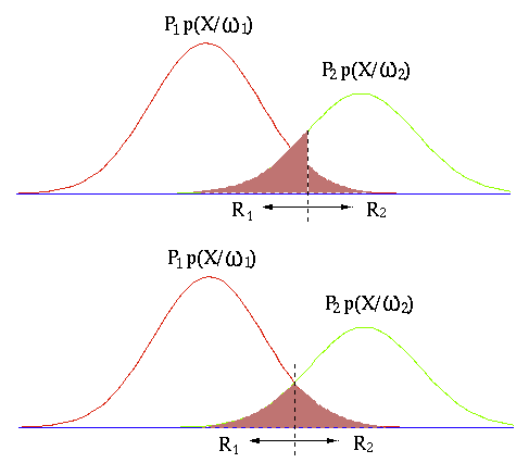
It is obvious that the Bayes classifier is indeed optimal, due to the fact that its boundary $p({\bf x}\vert C_i)P_i=p({\bf x}\vert C_j)P_j$ between classes $C_i$ and $C_j$ (the bottom plot) guarantees the classification error (shaded area) to be minimum.

To find the likelihood function $p({\bf x}\vert C_k)={\cal N}({\bf x},{\bf m}_k,{\bf\Sigma}_k)$, we need to find ${\bf m}_k$ and ${\bf\Sigma}_k$ based on the training set ${\cal D}=\{{\bf X},\,{\bf y}\}$, based on the $N_k$ training samples in class $C_k$ by the method of maximum likelihood estimation:

$${\bf m}_k=\frac{1}{N_k}\sum_{i=1}^{N_k} {\bf x}_i, \;\;\;\;\;\; {... ...k} ({\bf x}_i-{\bf m}_k)({\bf x}_i-{\bf m}_k)^T, \;\;\;\;\;\;({\bf x}_i\in C_k)$$ (14)

Once both $P_k=N_k/N$ and $p({\bf x}\vert C_k)={\cal N}({\bf x},{\bf m}_k,{\bf\Sigma}_k)$ are available, the classifier is trained, and the posterior $P(C_k\vert{\bf x})$ can be calculated for the classification in Eq. (12).

As the classification is based on the relative comparison of the posterior $P(C_k\vert{\bf x})$, any monotonic mapping of the posterior can be equivalently used to simplify the computation, such as the logarithmic function:

$$\log P(C_k\vert{\bf x}) = \log \left[ p({\bf x}\vert C_k) P_k/p({\bf x}) \right] =\log p({\bf x}\vert C_k) +\log P_k-\log p({\bf x})$$

$$= -\frac{1}{2}({\bf x}-{\bf m}_k)^T{\bf\Sigma}_k^{-1}({\bf x}-{\bf ... ...}{2}\log(2\pi)-\frac{1}{2}\log\vert{\bf\Sigma}_k\vert +\log P_k-\log p({\bf x})$$ (15)

Dropping the constant terms $\log p({\bf x})$ and $N \log(2\pi)/2$ that are independent of the index $k$ and therefore play no role in the comparison above, we get the quadratic discriminant function:

$$D_k({\bf x})=-\frac{1}{2}({\bf x}-{\bf m}_k)^T{\bf\Sigma}_k^{-1}({\bf x}-{\bf m}_k) -\frac{1}{2}\log\vert{\bf\Sigma}_k\vert+\log P_k$$ (16)

Now the classification can be represented by

$$\;\; D_l({\bf x})=\max \{ D_k({\bf x}),\;(k=1,\cdots,K)\}, \;\;\;\;\; \;\;{\bf x}\in C_l$$ (17)

Equivalently, we can also treat the negative of this discriminant function as a distance measurement:

$$d_k({\bf x})=({\bf x}-{\bf m}_k)^T{\bf\Sigma}_k^{-1}({\bf x}-{\bf m}_k) +\log\vert{\bf\Sigma}_k\vert-2\,\log P_k$$ (18)

for minimum distance classification. We note that the first term is the Mohalanobis distance defined previously. However, the additonal terms in the expression contribute to better classification performance.

Geometrically, the feature space is partitioned into regions corresponding to the $K$ classes by the decision boundaries between every pair of classes $C_i$ and $C_j$, represented by the equation $D_i({\bf x})=D_j({\bf x})$, i.e.,

$$-\frac{1}{2}({\bf x}-{\bf m}_i)^T{\bf\Sigma}_i^{-1}({\bf x}-{\bf m}_i) -\frac{1}{2}\;\log\,\vert{\bf\Sigma}_i \vert + \log\, P_i$$

$$= -\frac{1}{2}({\bf x}-{\bf m}_j)^T{\bf\Sigma}_j^{-1}({\bf x}-{\bf m}_j) -\frac{1}{2}\;\log\,\vert{\bf\Sigma}_j \vert + \log\, P_j$$ (19)

which can be written as

$${\bf x}^T{\bf W}{\bf x}+{\bf w}^T{\bf x}+w=0$$ (20)

where

$${\bf W} = -\frac{1}{2}({\bf\Sigma}_i^{-1}-{\bf\Sigma}_j^{-1})$$

$${\bf w} = {\bf\Sigma}_i^{-1}{\bf m}_i-{\bf\Sigma}_j^{-1}{\bf m}_j$$

$$w = -\frac{1}{2}({\bf m}_i^T{\bf\Sigma}_i^{-1}{\bf m}_i-{\bf m}_j^T{\... ...,\frac{\vert{\bf\Sigma}_i\vert}{\vert{\bf\Sigma}_j\vert} +\log\,\frac{P_i}{P_j}$$ (21)

In general, this decision boundary is a quadratic hypersurface (hypersphere, hyperellipsoid, hyperparabola, or hyperhyperbola), by which an unlabeled data sample ${\bf x}$ is classified into either of the two classes $C_i$ and $C_j$ based on whether it is on the positive or negative side of the surface::

$$\;\;{\bf x}^T{\bf W}{\bf x}+{\bf w}^T{\bf x}+w \left\{\begin{array}{l}>0\\ <0\end{array}\right.,\;\;\;\;\; \;\;\; {\bf x}\in \left\{\begin{array}{c} C_i\\ C_j \end{array}\right.$$ (22)

We further consider several special cases:

• All classes have the same prior:

  $$P_i=P_j\;\;\;\;(i,j=1,\cdots,K)$$ (23)

  then the last term of $D_i({\bf x})$ is zero, and we have

  $$D_i({\bf x})=-\frac{1}{2}({\bf x}-{\bf m}_i)^T{\bf\Sigma}_i^{-1}({\bf x}-{\bf m}_i) -\frac{1}{2}\;\log\,\vert{\bf\Sigma}_i \vert$$ (24)

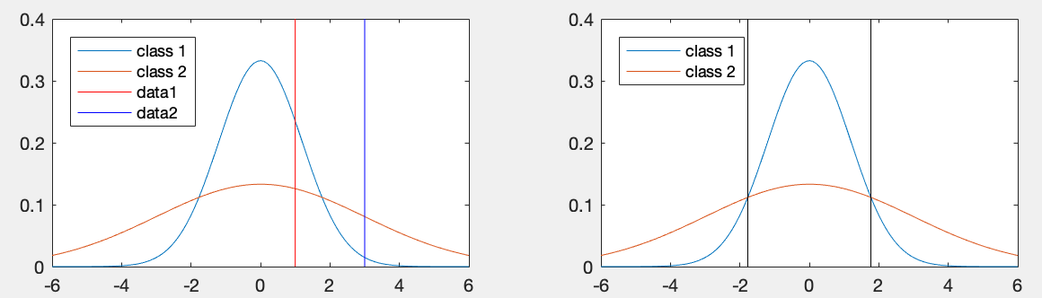
  We can reconsider Example 2 in the previous section but now based on the negative of the discriminant function above treated as a distance $d({\bf x},\,C_i)=({\bf x}-{\bf m}_i)^T{\bf\Sigma}_i^{-1}({\bf x}-{\bf m}_i) +\log\,\vert{\bf\Sigma}_i \vert$, and get

  $$\left\{ \begin{array}{l} d(x_1,\,C_1)=0.69+\log(1.2^2)=1.06, \;\;... ...\;\;\;\;\;\;\;\;\;\;\;\;\;\; d_M(x_1,\,C_2)=1+\log(3^2)=3.20 \end{array}\right.$$ (25)

  Now we see that $x_1$ is classified into class $C_1$, while $x_2$ into $C_2$, as desired. The misclassification of $x_1$ to $C_2$ by the Mahalanobis distance, the first term, is corrected, due to the addition of the second term $\log(\sigma^2)$. The plot below shows the partitioning of the 1-D space for the two classes $C_1$ and $C_2$:

  

• All classes have the same covariance matrix ${\bf\Sigma}_i={\bf\Sigma}$, the discriminant function becomes:

  $$D_i({\bf x})=-\frac{1}{2}({\bf x}-{\bf m}_i)^T{\bf\Sigma}^{-1}({\bf x}-{\bf m}_i) +\log\,P_i$$ (26)

  Moreover, if all $P_i$ are the same and the second term is dropped, $D_i({\bf x})$ becomes the negative Mahalanobis distance.

  The boundary equation $D_i({\bf x})=D_j({\bf x})$ between $C_i$ and $C_j$ becomes

  $$-\frac{1}{2}({\bf x}-{\bf m}_i)^T{\bf\Sigma}^{-1}({\bf x}-{\bf m}... ...=-\frac{1}{2}({\bf x}-{\bf m}_j)^T{\bf\Sigma}^{-1}({\bf x}-{\bf m}_j)+\log\,P_j$$ (27)

  As the quadratic terms ${\bf x}^T{\bf\Sigma}^{-1}{\bf x}$ on both sides of the equation are the same, it becomes a linear equation:

  $${\bf w}^T{\bf x}+w=0$$ (28)

  where

  $${\bf w}={\bf\Sigma}^{-1}({\bf m}_i-{\bf m}_j)$$ (29)

  and

  $$w=-\frac{1}{2}({\bf m}_i^T{\bf\Sigma}^{-1}{\bf m}_i -{\bf m}_j^T{\bf\Sigma}^{-1}{\bf m}_j)+\log\,\frac{P_i}{P_j}$$ (30)

  This linear equation represents a hyperplane between the two points ${\bf m}_i$ and ${\bf m}_j$ and perpendicular to the straight line ${\bf\Sigma}^{-1}({\bf m}_i-{\bf m}_j)$ (the straight line ${\bf m}_i-{\bf m}_j$ rotated by matrix ${\bf\Sigma}^{-1}$).

• All classes have the same isotropic distribution:

  $${\bf\Sigma}_i={\bf\sigma}^2\,{\bf I}=diag[\sigma^2,\cdots,\sigma^2]$$ (31)

  then $\vert{\bf\Sigma}_i\vert=\sigma^{2d}$ and $D_i({\bf x})$ becomes

  $$D_i({\bf x})=-\frac{\vert\vert {\bf x}-{\bf m}_i \vert\vert^2}{2\sigma^2}+\log\,P_i$$ (32)

  Note that the term $\log\,\vert{\bf\Sigma}_i\vert$ has been dropped from the original expression of $D_i({\bf x})$ as it is now the same for all classes.

  The boundary equation $D_i({\bf x})=D_j({\bf x})$ becomes:

  $$\frac{\vert\vert {\bf x}-{\bf m}_i \vert\vert^2}{2\sigma^2}-\log\,P_i =\frac{\vert\vert {\bf x}-{\bf m}_j \vert\vert^2}{2\sigma^2}-\log\,P_j$$ (33)

  which can be simplified to a linear equation:

  $${\bf w}^T{\bf x}+w=0$$ (34)

  where

  $${\bf w}={\bf m}_i-{\bf m}_j,\;\;\;\;\; w=-({\bf m}_i^T{\bf m}_i-{\bf m}_j^T{\bf m}_j)+2\sigma^2\;\log\,\frac{P_i}{P_j}$$ (35)

  This linear equation represents a hyperplane between the two points ${\bf m}_i$ and ${\bf m}_j$ and perpendicular to the straight line passing through these points.

• Further, if all classes have the same $P_i$, $D_i({\bf x})$ becomes

  $$D_i({\bf x})=-({\bf x}-{\bf m}_i)^T({\bf x}-{\bf m}_i)=-\vert\vert{\bf x}-{\bf m}_i\vert\vert^2$$ (36)

  and the Bayes classifier becomes minimum distance classifier based on Euclidean distance (maximizing $D_i({\bf x})$ is equivalent to minimizing $\vert\vert{\bf x}-{\bf m}_i\vert\vert^2$.

The Matlab functions for training and testing are listed low:

function [M S P]=NBtraining(X,y)        % naive Bayes training    
    [d N]=size(X);              	% dimensions of dataset
    K=length(unique(y));                % number of classes
    M=zeros(d,K);                       % mean vectors
    S=zeros(d,d,K);                     % covariance matrices
    P=zeros(1,K);                       % prior probabilities
    for k=1:K
        idx=find(y==k);                 % indices of samples in kth class 
        Xk=X(:,idx);                    % all samples in kth class
        P(k)=length(idx)/N;             % prior probability
        M(:,k)=mean(Xk');               % mean vector of kth class
        S(:,:,k)=cov(Xk');              % covariance matrix of kth class
    end
end

function yhat=NBtesting(X,M,S,P)        % naive Bayes testing
    [d N]=size(X);                      % dimensions of dataset
    K=length(P);                        % number of classes
    for k=1:K
        InvS(:,:,k)=inv(S(:,:,k));      % inverse of covariance matrix
        Det(k)=det(S(:,:,k));           % determinant of covariance matrix
    end
    for n=1:N                           % for each of N samples
        x=X(:,n);
        dmax=-inf;
        for k=1:K
            xm=x-M(:,k);
            d=-(xm'*InvS(:,:,k)*xm)/2;
            d=d-log(Det(k))/2+log(P(k));  % discriminant function
            if d>dmax
                yhat(n)=k;              % assign nth sample to kth class
                dmax=d;
            end
        end       
    end
end

The classification result in terms of the estimated class identity $\hat{\bf y}$ of the training samples compared with the ground truth class labeling ${\bf y}$ can be represented in the form of a $K\times K$ confusion matrix, of which the element in the ith row and jth column is the number of training samples labeled as a member of the ith class but actually classified into the jth class. For an ideal classifier that classifies all data samples correctly, this confussion matrix should be a diagonal matrix. But for a nonideal classifier, its error rate can be found as the percentage of the number of misclassified samples (sum of all off-diagonal elements) out of the total number of samples. The code below shows the function that generates such a confussion matrix based on the estimated class identity $\hat{\bf y}$ and the ground truth labeling ${\bf y}$:

function [Cm er]=ConfusionMatrix(yhat,ytrain)
    N=length(ytrain);                 % number of test samples
    K=length(unique(ytrain));         % number of classes
    Cm=zeros(K);                      % the confussion matrixxs
    for n=1:N
        i=ytrain(n);
        j=yhat(n);
        Cm(i,j)=Cm(i,j)+1;                
    end
    er=1-sum(diag(Cm))/N;             % error percentage
end

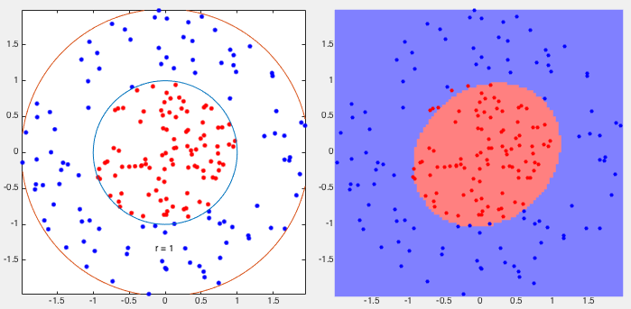
Example 1:

This example shows the classification of two cocentric classes with one surrounding the other. They are separated by an ellipse with 9 out of 200 samples misclassified, i.e., the error rate of $9/200=4.5\%$. The confusion matrix is shown below:

$$\left[\begin{array}{rrr} 92 & 8 \\ 1 & 99 \\ \end{array}\right]$$ (37)

indicating 8 of the 100 samples belonging to class 1 are misclassified to class 2, and 1 of the 100 samples belonging to class 2 is misclassified to class 1.

Example 2:

This example shows the classification of a 2-class exclusive-or (XOR) data set with significant overlap, in terms of the confusion matrix and the error rate of $61/400=15.25\%$. Note that the decision boundaries are a pair of hyperbolas. The confusion matrix is

$$\left[\begin{array}{rrr} 175 & 25 \\ 36 & 164 \\ \end{array}\right]$$ (38)

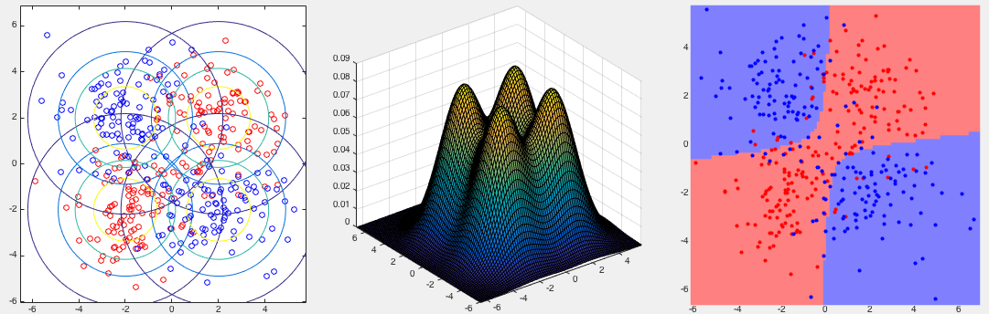
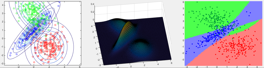
Example 3:

The first two panels in the figure below show three classes in the 2-D space, while the third one shows the partitioning of the space corresponding to the three classes. Note that the boundaries between the classes are all quadratic. The confusion matrix of the classification result is shown below, with the error rate $49/600=8.17\%$.

$$\left[\begin{array}{rrr} 196 & 3 & 1 \\ 0 & 191 & 9 \\ 3 & 33 & 164 \\ \end{array}\right]$$ (39)

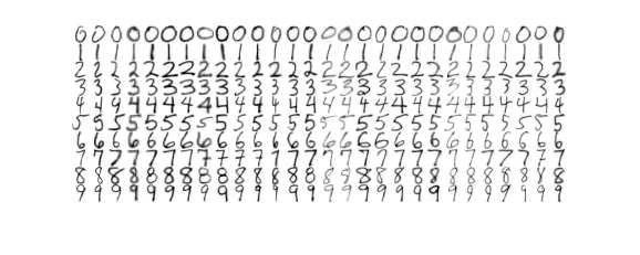
Example 4

The figure below shows some sub-samples of ten sets digits from 0 to 9, each is hand-written 224 times by different students. Each hand-written digit is represented as an 16 by 16 image containing 256 pixels, treated as a 256 dimensional vector.

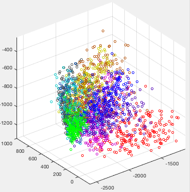
The dataset can be visualized by applying the KLT transform to map all data points in the 256-D space into a 3-D space spanned by the three eigenvectors corresponding to the three greatest eigenvalues of the covariance matrix of the dataset, as shown below:

The naive Bayes classifier is applied to the dataset of handwritten digits from 0 to 9, of which each data sample is a 256-dimensional vector composed of $16\times 16$ pixels of an image for the handwritten of a digit. The dataset contains 224 samples per class and $N=2240$ in total for all $K=10$ classes.

We note that the 256-dimensional covariance matrix ${\bf\Sigma}_k$ for each of the $K=10$ classes is estimated by the 224 samples in the class, i.e., the estimated covariance matrix does not have a full rank and is not invertible. This issue can be resolved by applying KLT to the dataset to reduce its dimensionality from 256 to some value smaller than 224, such as 100.

The classifier is trained on half of the dataset of 1120 randomly selected samples and then tested on the remaining 1120 samples. The classification results are given below in terms of the confusion matrices of the traing samples (left) and the testing samples (right). All 1120 training samples are correctly classfied, while out of the remaining 1120 test samples, 198 are misclassified ($17.7\%$ error).

$$\left[ \begin{array}{rrrrrrrrrr} 107 & 0 & 0 & 0 & 0 & 0 & 0 & 0 ... ... 18 & 109 & 9 \\ 0 & 3 & 0 & 0 & 2 & 0 & 0 & 2 & 0 & 90 \\ \end{array}\right]$$ (40)