Next: Bayesian Linear Regression Up: Regression Analysis and Classification Previous: Bias-Variance Tradeoff and Ridge
The method of linear regression considered previously can
be generalized to model nonlinear relationships between
the dependent variable  and the independent variables
in
and the independent variables
in
![${\bf x}=[x_1,\cdots,x_d]^T$](img491.svg) by a regression function
as a linear combination of
by a regression function
as a linear combination of  nonlinear basis functions
of
nonlinear basis functions
of  :
:
 |
(145) |
 is
the basis functions parameterized by
is
the basis functions parameterized by
 that
span the function space in which
that
span the function space in which  resides. Some
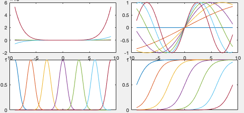
of the common basis functions include the following:
resides. Some
of the common basis functions include the following:
 |
(146) |
 is
is  th order polynomial
function.
th order polynomial
function.
 or or |
(147) |
is similar to the sine or
cosine series expansion of the given function.
 |
(148) |
 .
.
 |
(149) |
The original d-dimensional data space spanned by
 is now converted to a K-dimensional space spanned by the basis
functions
is now converted to a K-dimensional space spanned by the basis
functions
 . Applying
such a regression model to each data point
. Applying
such a regression model to each data point  , we get
 |
(150) |
 is a
is a  matrix of which the
component in the nth row and kth column is the kth basis
function evaluated at the nth data point:
Typically there are many more sample data points than the basis
functions, i.e.,
matrix of which the
component in the nth row and kth column is the kth basis
function evaluated at the nth data point:
Typically there are many more sample data points than the basis
functions, i.e.,  .
.
As the nonlinear model
 in
Eq. (151) is in the same form as the linear model
in
Eq. (151) is in the same form as the linear model
 in Eq. (108),
we can solve it to find the LS solution
in Eq. (108),
we can solve it to find the LS solution  the same
way as in Eq. (116), by simply replacing
the same
way as in Eq. (116), by simply replacing  by
:
by
:
 is the
pseudo-inverse
of the
is the
pseudo-inverse
of the  matrix
 . Now we get the output
of the regression model
. Now we get the output
of the regression model
 |
(154) |
The Matlab code segment belows shows the essential part
of the algorithm, where  is the nth data sample
out of the total of
is the nth data sample
out of the total of  ,
,  represents
vector
represents
vector
![${\bf y}=[y_1,\cdots,y_N]^T$](img499.svg) with
with
 ,
and
,
and  represents the parameters for the kth basis
function
represents the parameters for the kth basis
function
 .
.
     for n=1:N
         for k=1:K
             Phi(n,k)=phi(x(n),c(k));
         end
     end
     w=pinv(Phi)*y(x);    	% weight vector by LS method
     yhat=Phi*w;                % reconstructed function
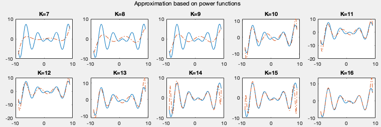
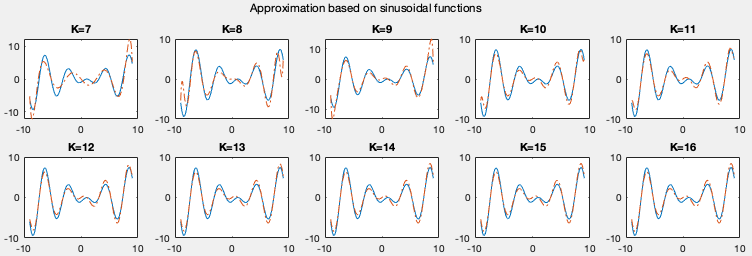
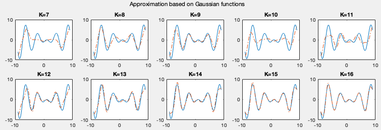
Example:
The plots below show the approximations of a function using linear regression based on four different types of basis functions listed above. We see that the more basis functions are used, the more accurately the given funtion is approximated.
Example:
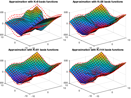
The plots below show the approximations of a 2-D function
 shown below using linear regression
based on Gaussian basis functions centered at different
locations in the 2-D space.
shown below using linear regression
based on Gaussian basis functions centered at different
locations in the 2-D space.
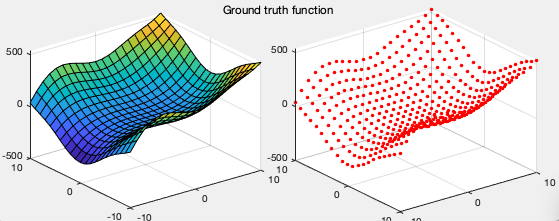
The figure below shows a 2-D function (left) and the
sample points (right) used for regression:
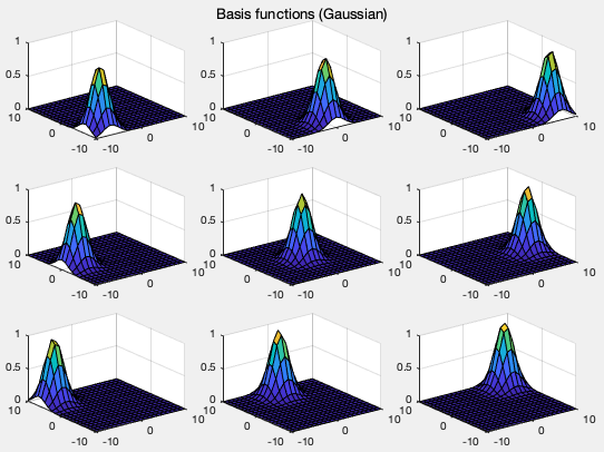
The figure below shows  Gaussian basis functions
located at different locations in the 2-D space:
Gaussian basis functions
located at different locations in the 2-D space:
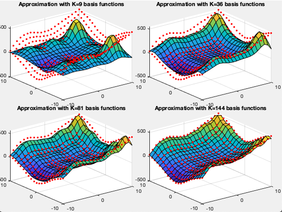
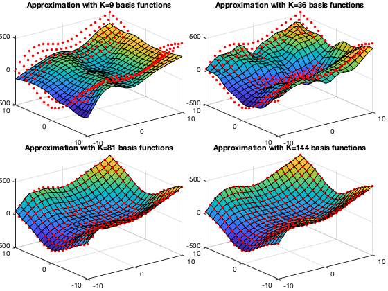
The figure below shows the approximated functions
based on different number of basis functions:
In addition to the different types of basis functions listed above, we further consider the following basis functions:
where in, called activation function, can take
some different forms such as
in, called activation function, can take
some different forms such as
 |
(156) |
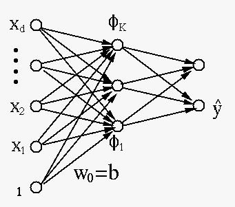
As shown in figure, the  nodes of the input layer take
the components of one of the data points as
inputs, and each of the nodes of the hidden layer finds
the linear combination
nodes of the input layer take
the components of one of the data points as
inputs, and each of the nodes of the hidden layer finds
the linear combination
 of these
components from the input layer together with a bias term
of these
components from the input layer together with a bias term
 , and generates an output
 .
A node of the output layer in tern takes the outputs from
the nodes in the hidden layer and generates an output
.
A node of the output layer in tern takes the outputs from
the nodes in the hidden layer and generates an output
 as the regression approximation of the desired function
 . Note that there exist two sets of weights
here, those in vector
. Note that there exist two sets of weights
here, those in vector  for each of the hidden
layer nodes, and those for the node of the output layer found
in Eq. (153). If there are multiple
nodes in the output layer, they can each approximate a
different function. This three-layer network is of particular
interest in neural network algorithms, to be considered in
Chapter 9.
///
for each of the hidden
layer nodes, and those for the node of the output layer found
in Eq. (153). If there are multiple
nodes in the output layer, they can each approximate a
different function. This three-layer network is of particular
interest in neural network algorithms, to be considered in
Chapter 9.
///
Example
This method of regression based on basis functions is applied
to approximating the same 2-D function
in the previous example, as a linear combination of basis
functions
 with each
parameterized by and . The regression is based
on a set of data samples
with each
parameterized by and . The regression is based
on a set of data samples
 taken from a grid of the 2-D space, and the corresponding
function values in
taken from a grid of the 2-D space, and the corresponding
function values in
 .
.
The Matlab code segment below shows the essential part
of the program for this example, where  is a function
to be approxmiated, which can be arbitrarily specified.
is a function
to be approxmiated, which can be arbitrarily specified.
    g=@(x) x.*(x>0);        % ReLU activation function, or
    g=@(x) 1/(1+exp(-x));   % Sigmoid activation function
    g=@(x,w,b)g(w'*x+b);    % the basis function

    [X,Y]=meshgrid(xmin:1:xmax, ymin:1:ymax); % define 2-D points
    nx=size(X,2);           % number of samples in first dimension
    ny=size(Y,1);           % number of samples in second dimension
    N=nx*ny;                % total number of data samples
    Phi=zeros(N,K);   	    % K basis functions evaluated at N sample points
    W=1-2*rand(2,K);        % random initialization of weights
    b=1-2*rand(1,K);        % and biases for K basis functions
    n=0;
    for i=1:nx
        x(1)=X(1,i);        % first component
        for j=1:ny
            x(2)=Y(j,1);    % second component
            n=n+1;          % of the nth sample
            Y(i,j)=func(x); % function evalued at the sample
            for k=1:K       % basis functions evaluated at the sample
                Phi(n,k)=g(x,W(:,k),b(k));
            end
        end
    end
    y=reshape(Y,N,1);       % convert function values to vector
    w=pinv(Phi)*y;    	    % find weights by LS method
    yhat=Phi*w;             % reconstructed function
    Yhat=reshape(yhat,m,n); % convert vector y to 2-D to compare w/ Y
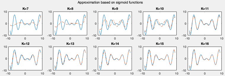
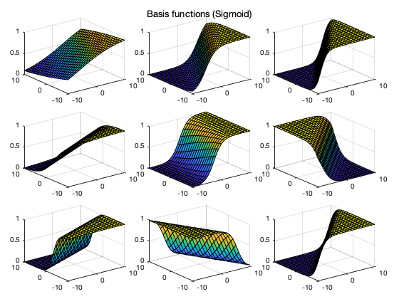
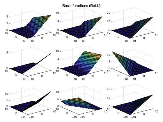
The figures below show the regression results as well as the basis functions used, based on both the sigmoid and ReLU activation functions. We note that as the function is better approximated when more basis functions are used in the regression.
![$\displaystyle \hat{\bf y}
=\left[\begin{array}{c}y_1\\ \vdots\\ y_N\end{array}\...
...
\left[\begin{array}{c}w_1\\ \vdots\\ w_K\end{array}\right]
={\bf\Phi}^T{\bf w}$](img744.svg)
![$\displaystyle {\bf\Phi}=\left[\begin{array}{ccc}
\varphi_1({\bf x}_1)&\cdots&\v...
...ts&\vdots\\
\varphi_1({\bf x}_N)&\cdots&\varphi_K({\bf x}_N)\end{array}\right]$](img747.svg)

