Kernel Mapping

The SVM algorithm above converges only if the data points of the two classes in the training set are linearly separable. If this is not the case, we can consider the following kernel method.

In the kernel method, all data points as a vector ${\bf x}=[x_1,\cdots,x_d]^T$ in the original d-dimensional feature space are mapped by a kernel function ${\bf z}=\phi({\bf x})$ into a higher, possibly infinite, dimensional space

$${\bf x} \Longrightarrow {\bf z}=\phi({\bf x})$$ (94)

The presumption of the method is that the data points only appear in the form of inner product ${\bf x}_m^T{\bf x}_n$ in the algorithm, and the kernel function ${\bf z}=\phi({\bf x})$ never needs to be actually carried out. In fact, the form of the kernel function $\phi({\bf x})$ and the dimensionality of the higher dimensional space do not need to be explicitly specified or known.

The motivation for such a kernel mapping is that the relevant operations such as classification and clustering may be carried out much more effectively once the dataset is mapped to the higher dimensional space. For example, classes not linearly separable in the original d-dimensional feature space may be trivially separable in a higher dimensional space, as illustrated by the following examples.

Example 1

In 1-D space, classes $C_-=\{x\big\vert(a\le x\le b)\}$ and $C_+=\{x\big\vert(x\le a)\;$or$\;(x\ge b)\}$ are not linearly separable. By the following mappping from 1-D space to 2-D space:

$${\bf z}=\phi(x)=\left[\begin{array}{l}z_1\\ z_2\end{array}\right] =\left[ \begin{array}{c} x \\ (x-(a+b)/2)^2 \end{array}\right]$$ (95)

the two classes can be separated by a threshold in the second dimension of the 2-D space.

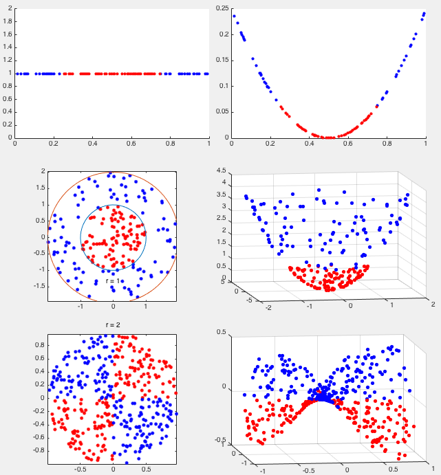
Example 2:

The method above can be generalized to higher dimensional spaces such as mapping from 2-D to 3-D space. Consider two classes in a 2-D space that are not linearly separable: $C_-=\{{\bf x},\; \vert\vert{\bf x}\vert\vert< D\}$ and $C_+=\{{\bf x},\; \vert\vert{\bf x}\vert\vert> D\}$. However, by the following mappping from 2-D space to 3-D space:

$${\bf z}=\phi({\bf x})=\left[\begin{array}{l}z_1\\ z_2\\ z_3\end{array}\right] =\left[\begin{array}{c}x_1\\ x_2\\ x_1^2+x_2^2\end{array}\right]$$ (96)

the two classes can be trivially separated linearly by thresholding in the third dimension of the 3-D space.

Example 3:

In 2-D space, in the exclusive OR data set, the two classes of $C_-$ containing points in quadrants I and III, and $C_+$ containing points in quadrants II and IV are not linearly separable. However, by mapping the data points to a 3-D space:

$${\bf z}=\phi({\bf x})=\left[\begin{array}{l}z_1\\ z_2\\ z_3\end{array}\right] =\left[\begin{array}{c}x_1\\ x_2\\ x_1x_2\end{array}\right]$$ (97)

the two classes can be separated by simply thresholding in the third dimension of the 3-D space.

Definition: A kernel is a function that takes two vectors ${\bf x}_m$ and ${\bf x}_n$ as arguments and returns the inner product of their images ${\bf z}_m=\phi({\bf x}_m)$ and ${\bf z}_n=\phi({\bf x}_n)$:

$$K({\bf x}_m,{\bf x}_n)=\phi({\bf x}_m)^T\phi({\bf x}_n) ={\bf z}_m^T{\bf z}_n$$ (98)

The kernel function takes as input some two vectors ${\bf x}_m$ and ${\bf x}_n$ in the original feature space, and returns a scalor value as the inner product ${\bf z}_m$ and ${\bf z}_n$ in some higher dimensional space. If the data points in the original space only appear in the form of inner product, then the kernel function ${\bf z}=\phi({\bf x})$, called the kernel-induced implicit mapping, never needs to be explicitly specified, and the dimension of the new does not even need to be known.

The following is a set of commonly used kernel functions $K({\bf x},\,{\bf x}')$, which can be represented as an inner product of two vectors ${\bf z}=\phi({\bf x})$ and ${\bf z}'=\phi({\bf x}')$ in a higher dimensional space.

• linear kernel (no kernel mapping)

  Assume ${\bf x}=[x_1,\cdots,x_d]^T$, ${\bf x}'=[x'_1,\cdots,x'_d]^T$,

  $$K({\bf x},{\bf x}')={\bf x}^T {\bf x}'=\sum_{i=1}^d x_ix'_i$$ (99)

• polynomial kernels

  The binomial theorem states:

  $$(x+y)^n=\sum_{k=0}^n\left(\begin{array}{c}n\\ k\end{array}\right) x^{n-k} y^k =\sum_{k=0}^n \frac{n!}{k!(n-k)!}\; x^{n-k} y^k$$ (100)

  where the binomial coefficient

  $$\left(\begin{array}{c}n\\ k\end{array}\right)=\frac{n!}{k!(n-k)!}$$ (101)

  is the number of ways to distribute $n$ items into two bins ($k$ in one and $n-k$ in the other). This result can be generalized to the multinormial case:

  $$(x_1+\cdots+x_d)^n=\sum_{\sum_{i=1}^d k_i=n} \left(\begin{array}{... ...} =\sum_{\sum_{i=1}^d k_i=n}\frac{n!}{k_1!\cdots k_d!}x_1^{k_1}\cdots x_d^{k_d}$$ (102)

  where the multinomial coefficient

  $$\left(\begin{array}{c}n\\ k_1,\cdots,k_d\end{array}\right) =\frac{n!}{k_1!\cdots k_d!}$$ (103)

  is the number of ways to distribute $n$ balls into $d$ bins with $k_i$ balls in the ith bin (see here), and the summation is over all possible ways to get $d$ non-negative integers $k_1,\cdots,k_d$ that add up to $n$.

  Now consider the homogeneous polynomial kernel for d-dimensional vectors ${\bf x}=[x_1,\cdots,x_d]^T$ defined as
  

  $$K({\bf x},{\bf x}') = ({\bf x}^T{\bf x}')^n=(x_1x'_1+\cdots+x_dx'_d)^n$$

  $$= \sum_{\sum_{i=1}^d k_i=n}\frac{n!}{k_1!\cdots k_d!}\; \left( (x_1... ...cdots (x_dx'_d)^{k_d} \right) =\phi({\bf x})^T \phi({\bf x}')={\bf z}^T{\bf z}'$$ (104)

  
  where

  $${\bf z}=\phi({\bf x})=\left[\sqrt{ \frac{n!}{k_1!\cdots k_d!} } \... ...1}\cdots x_d^{k_d}\right),\;\left(k_i\ge 0,\;\sum_{i=1}^d k_i=n\right)\right]^T$$ (105)

  In particular, when $d=2$ and $n=2$, the polynomial kernel defined over 2-D vectors ${\bf x}=[x_1,x_2]^T$ is:

  $$K({\bf x},{\bf x}')=({\bf x}^T{\bf x}')^2=(x_1x'_1+x_2x'_2)^2 =(x... ..._1 x'_1 x_2 x'_2+(x_2 x'_2)^2=\phi({\bf x})^T \phi({\bf x}') ={\bf z}^T{\bf z}'$$ (106)

  where ${\bf z}=\phi({\bf x})=[x_1^2,\,\sqrt{2}x_1x_2,\,x_2^2]$ is a mapping from ${\bf x}$ in 2-D space to ${\bf z}$ in 3-D space.

  A non-homogeneous polynomial kernel is defined as

  $$K({\bf x},{\bf x}')=(1+{\bf x}^T{\bf x}')^n$$ (107)

• The radial basis function (RBF) kernel

  The RBF kernel is defined as

  $$K({\bf x},{\bf x}')=e^{-\vert\vert{\bf x}-{\bf x}'\vert\vert^2/2\sigma^2} =e^{-\gamma\vert\vert{\bf x}-{\bf x}'\vert\vert^2}$$ (108)

  where $\gamma=1/2\sigma^2$ is a parameter that can be adjusted to fit each specific dataset. This kernel can be wriiten as the inner product of two infinite dimensional vectors (for simplicity, we assume $\sigma=1$):
  

  $$K({\bf x},\,{\bf x}') = e^{-\vert\vert{\bf x}-{\bf x}'\vert\vert^2/2} =e^{-\vert\vert{\bf... ...\vert{\bf x}'\vert\vert^2/2} \sum_{n=0}^\infty \frac{({\bf x}^T{\bf x}')^n}{n!}$$

  $$= e^{-\vert\vert{\bf x}\vert\vert^2/2} \; e^{-\vert\vert{\bf x}'\ve... ...!}{k_1!\cdots k_d! } \left((x_1x'_1)^{k_1}\cdots (x_dx'_d)^{k_d}\right) \right]$$

  $$= \sum_{n=0}^\infty \sum_{\sum_{i=1}^d k_i=n} \left(e^{-\vert\vert{... ...; \frac{x_1^{\prime k_1}\cdots x_d^{\prime k_d}}{\sqrt{k_1!\cdots k_d!}}\right)$$

  $$= \phi({\bf x})^T \phi({\bf x}')={\bf z}^T{\bf z}'$$ (109)

  
  where

  $${\bf z}=\phi({\bf x})=\left[ e^{-\vert\vert{\bf x}\vert\vert^2/2}... ...1!\cdots k_d!}}, \;\left(n=0,\cdots,\infty,\;\sum_{k=1}^nk_i=n\right) \right]^T$$ (110)

  is a vector in an infinite dimensional space. In particular, when $d=1$ we have
  

  $$K(x,\,x') = e^{-(x-x')^2/2}=e^{-x^2/2}\, e^{-x'^2/2}\, e^{xx'} =e^{-x^2/2}\, e^{-x'^2/2} \sum_{n=0}^\infty \frac{(xx')^n}{n!}$$

  $$= \sum_{n=0}^\infty (e^{-x^2/2}\,x^n/\sqrt{n!})\;(e^{-x'^2/2}\,x'^n/\sqrt{n!})$$ (111)

  
  where ${\bf z}=\phi(x)=\left[ e^{-x^2/2}\,x^n/\sqrt{n!}, \;(n=0,\cdots,\infty)\right]^T$ is a kernel function that maps a 1-D space into an infinite dimensional space.

The method of kernel mapping can be applied to the SVM algorithm consider previously as all data points appear in the algorithm are in the form of an inner product. Specifically, during the training process, we replace the inner product ${\bf x}_m^T{\bf x}_n$ in both Eq. (85) and Eq. (88) by the kernel functioin $K({\bf x}_m,\,{\bf x}_n)$ to get

$$\;\; L_d({\bf\alpha}) =\sum_{n=1}^N\alpha_n -\frac{1}{2} \sum_{n=1}^N \sum_{m=1}^N \alpha_n \alpha_m y_n y_m K({\bf x}_n,{\bf x}_m)$$

$$\;\; \sum_{n=1}^N \alpha_n y_n ={\bf y}^T{\bf\alpha}=0, \;\;\;\; \alpha_n\ge 0\;\;\;(n=1,\cdots,N)$$ (112)

and

$$b=y_n-\sum_{m \in sv} \alpha_m y_m K({\bf x}_m,{\bf x}_n),\;\;\;\;\;(n\in sv)$$ (113)

We also replace the inner product ${\bf x}^T_n{\bf x}$ in Eq. (89) by $K({\bf x}_n,\,{\bf x})$ for the classification of any unlabeled point ${\bf z}=\phi({\bf x})$:

$$f({\bf z})={\bf w}^T{\bf z}+b =\sum_{n\in sv}\alpha_ny_n\,({\bf z... ...\{\begin{array}{ll}>0 & {\bf x}\in C_+\\ <0 & {\bf x}\in C_- \end{array}\right.$$ (114)

Again, we note that the normal vector ${\bf w}$ in Eq. (86) never needs to be explicitely calculated. As now both the training and classification are carried out in some higher dimensional space ${\bf z}=\phi({\bf x})$, in which the classes are more likely linearly separable, the classification can be more effectively. More generally, the kernel method can be applied to any algorithm, so long as the data always appear in the form of an inner product.