Model-Free Evaluation and Control

The previously discussed dynamic programming methods find the optimal policy based on the assumption that the MDP model of the environment is completely available, i.e., the dynamics of MDP in terms of its state transition and reward mechanism are known. A given policy $\pi$ can then be evaluated based the transition probabilities $p(s'\vert s, a)$, and improved based on greedy action selection at each state. Such a model-based optimization problem, called planning, involves no learning of the environment.

Now we consider the optimization problem with an unknown MDP model of the environment. In this model-free problem, called control, the state transition and reward probabilities of the MDP model are unknown, the value functions can no longer be calculated directly based on Eqs. (21) and (22) as in model-based planning. Instead, now we need to learn the MDP model by sampling the environment, i.e., by repeatedly running a large number of episodes of the stochastic process of the environment while following some given policy, and estimate the value functions as the average of the actual returns received during the sampling process. This method is generally referred to as Monte Carlo (MC) method. At the same time, the given policy can also be improved to gradually approach optimality.

This approach is called general policy iteration (GPI), as illustrated in Eq. (40) below, similar to the policy iteration (PI) algorithm for model-based planning illustrated in Eq. (37). In general, all model-free control algorithms are based on GPI by which the two alternating processes of policy evaluation and policy imprvement are carried out iteratively. This GPI can also be similarly illustrated in Fig. 1.3 for the GI.

$$\pi_o\stackrel{E}{\longrightarrow} q_{\pi_0}\stackrel{I}{\longrig... ...s \stackrel{I}{\longrightarrow}\pi^* \stackrel{E}{\longrightarrow}q_{\pi^*}=v^*$$ (40)

While GPI and GI illustrated in respectively in Eqs. (40) and (37) may look similar to each other, there are some essential differences between the two, as listed below.

• First, in model-free control the policy improvement is based on the action-value function $q_\pi(s,a)$, instead of the state value function $v_\pi(s)$ in model-based planning. This is because without the a specific MDP model the state value function can no longer be calculated, while the action value function can still be estimated based on the actual rewards received while sampling the environment. Similar to how we improve the policy by taking a greedy action to achive a higher state value in model-based planning, here we improve the policy by taking an action different from that dictated by the given policy $\pi$ to achieve a higher action value based on some $\epsilon$-greedy method, as discussed below.

• Second, as estimating the action value by the MC method requires running a large number of episodes while the sampling of the environment, the computational complexity for policy evaluation in the model-free case is much higher than that in model-based planning. To speed up this process in model-free control, the iterative policy evaluation is no longer fully carried for it to converge to the true action value of the policy. Instead, in model-free control, the iterative update of the action value is carried out only once, followed immediately by the next phase of policy improvement. Such an estimated action value is innevitably very noisy, but due to the much reduced complexity, we can afford to run a large number of sample episodes while sampling the envirionment.

• Third, in the PI process of model-based planning, the action value is found based on all available actions at each state (Eq. (22)) during policy evaluation, and we only need to exploit the greedy action at each state to find the policy that achieves the maximum action value $q_\pi(s)$ (Eq. (27)) during policy improvement. However, here in model-free control, we have to learn the action value $q_\pi(s,a)$, as a function of action $a\in A(s)$ as well as state $s$ by sampling the environment. Such an estimated action value based only on some partial sample data is inevitably noisy, especially in the early stage of learning when many of the states have not yet been visited yet. We therefore need to explore all actions at each state to better learn the value function, as well as to exploit the greedy action to improve the policy.

This issue of exploration versus exploitation can be addressed by the $\epsilon$-greedy method to make a proper trade-off between the exploitation of the greedy action and the exploration of other non-greedy actions, so that the agent can be exposed to all possible state-action pairs and gradually learn the action value function while at the same time also improve the policy being followed. In this method, we define $\epsilon\in[0,\;1]$ as the probability to explore any randomly chosen action $a\in\vert A(S)\vert$ out of all actions available in state $s$, each with an equal probability $\epsilon/\vert A(s)\vert$, and $1-\epsilon$ is the probability of taking the greedy action as one of the $\vert A(s)\vert$ actions, with probability $1-\epsilon+\epsilon/\vert A(s)\vert$.

$$\pi'(a\vert s) =\left\{\begin{array}{ll} \argmax_aq(s,a) & Pr=1-\... ...ert \\ \mbox{any $a\in A(s)$} & Pr=\epsilon/\vert A(s)\vert \end{array}\right.$$ (41)

For example, if $\vert A(s)\vert=4$ and $\epsilon=2/3$, the greedy action may be chosen with probability $1-\epsilon+\epsilon/\vert A(s)\vert=3/6$, while each of the remaining three non-greedy actions may be chosen with probability $\epsilon/\vert A(s)\vert=1/6$. Such a policy describes the behavior of the agent, and is therefore called behavior policy, different from the policy being followed.

We further note that a larger value of $\epsilon$ (close to 1) can be used to emphasize exploration at the early stage of the iteration when many state-action pairs have not been visited yet, while progressively smaller $\epsilon$ values (approaching to 0) can be used to amphasize exploitation for higher values in the later stage of the iteration when the action value function has been more reliably learned. For example, we can let $\epsilon_k=1/k$ be inversely proportional to the current number of iterations $k$, so that the larger $\epsilon$ values at the early stage of the iteration allow more sate-action pairs to be explored, while smaller $\epsilon$ values in the later stage of the iteration encourage exploitation of the greedy actions. To the limit $k\rightarrow\infty$ and $\epsilon\longrightarrow 0$, the $\epsilon$-greedy method approaches absolute greedy method.

Similar to how we proved the policy improvement theorem in Eq. (30) stating that the greedy policy $\pi'(s)$ achieves state value $v_{\pi'}(s)$ no lower than $v_\pi(s)$ achieved by the original policy $\pi$, i.e., $\pi'(s)\ge\pi(s)$, here we can also prove the same policy improvement theorem stating that the $\epsilon$-greedy policy $\pi'$ achieves action value $q_{\pi'}(s,a)$ no lower than $q_\pi(s,a)$ by the original policy $\pi$:

$$q_\pi(s,\pi'(s)) = \sum_a \pi'(a\vert s) q_\pi(s,a)$$

$$= \frac{\epsilon}{\vert A(s)\vert}\sum_aq_\pi(s,a)+ (1-\epsilon)\max_a q_\pi(s,a)$$

$$\ge \frac{\epsilon}{\vert A(s)\vert}\sum_aq_\pi(s,a)+ (1-\epsilon)\sum_a\frac{\pi(a\vert s)-\epsilon/\vert A(s)\vert} {1-\epsilon}q_\pi(s,a)$$ (42)

where the inequality is due to the fact that the maximum value of $q_\pi(s,a)$ is no less than the average of action values $q_\pi(s,a)$ over all $a\in A(s)$ weighted by some normalized coefficients adding up to 1:

$$\sum_a\frac{\pi(a\vert s)-\epsilon/\vert A(s)\vert}{1-\epsilon} =... ... s)-\frac{\epsilon}{\vert A(s)\vert}\right) =\frac{1}{1-\epsilon}(1-\epsilon)=1$$ (43)

Continuing the equation above we further get

$$q_\pi(s,\pi'(s)) \ge \frac{\epsilon}{\vert A(s)\vert}\sum_aq_\pi(s,a)- \frac{\epsilon}{\vert A(s)\vert}\sum_a q_\pi(s,a) +\sum_a\pi(a\vert s) q_\pi(s,a)$$

$$= \sum_a\pi(a\vert s) q_\pi(s,a)=v_\pi(s)$$ (44)

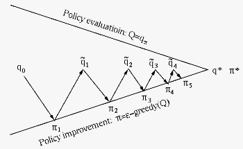
The iterative process of the GPI method for model-free control is illustrated in the figure below, similar to the PI method for model-based planning based planning illustrated in Fig. 1.3, but with the state value $v_\pi(s)$ replaced by the action value $q_\pi(s,a)$, and the greedy method replaced by $\epsilon$-greedy method.

Also, here the estimated action value $\tilde{q}$ is obtained with only one iteration for policy evaluation, instead of a much more accurate estimate that could otherwise be obtained if the iterative evaluation was fully carried out to its convergence (the top line). At the same the time, based on the estimated $\tilde{q}$ policy improvement is carried out by the $\epsilon$-greedy method (the bottom line).

The main task in model-free control is to evaluate the state and action-value functions given in Eqs. (21) and (22) while following a given policy $\pi$ without a specific MDP model. This is done by sampling of the dynamic process of the environment, and then estimating the value functions as the average of the actual returns received by the agent. Specifically, we run a large number of episodes (all assumed to terminate) of the MDP model of the environment by taking actions $a_t=\pi(s_t)$ in each state $s_t,\;(t=1,\cdots,T)$:

$$s_0\rightarrow(a_1,r_1,s_1)\rightarrow(a_2,r_2,s_2)\rightarrow \cdots\rightarrow(a_T,r_T,s_T)$$ (45)

and estimate the value functions based on the averaged returns $G_t$ actually received from these episodes.

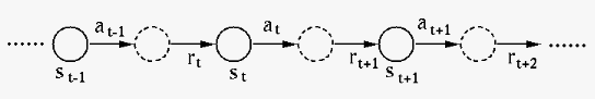
Such a sequence of states visited is called a trajectory, and the trajectories of different episodes are in general different from each another due to the random nature of the environment. In the following sections we will consider specific algoithms for the implementation of the general model-free control discussed above.

To prepare for specific discussion of the GPI methods, we first consider a general problem of the estimation of the value of a random variable $x$ as the running average of its samples beging collected in real time. Speicically the average $\hat{x}_n$ based on previous $n$ samples $x_1,\cdots,x_n$ is updated incrementally upon receiving a new sample $x_{n+1}$:

$$\hat{x}_{n+1} = \frac{1}{n+1}\sum_{i=1}^{n+1} x_i =\frac{1}{n+1}\left(x_{n+1}+\sum_{i=1}^n x_i\right)$$

$$= \frac{1}{n+1}(x_{n+1}+n\hat{x}_n) =\hat{x}_n+\frac{1}{n+1}(x_{n+1}-\hat{x}_n)$$ (46)

This running average can be generalized to

$$\hat{x}_{n+1}=\hat{x}_n+\alpha (x_{n+1}-\hat{x}_n)$$ (47)

This equation can be interpreted as

$$= + \times( - )$$ newEstimate

$$= + \times$$

$$= +$$ (48)

and considered as one iterative step in the method of stochastic gradient descent (SGD), for minimizing the squared error $\varepsilon=(x_{n+1}-\hat{x}_n)^2/2$ between the old average $\hat{x}_n$ and the latest sample $x_{n+1}$, and the second term is the gradient $d\varepsilon/d\hat{x}_n$ weighted by the step size $\alpha\in[0,\;1]$, which controls how samples are weighted differently. In the extreme case when $\alpha=1$, $\hat{x}_n=x_n$ with no contribution from any previous samples; on the other hand when $\alpha$ is close to 0, $\hat{x}_n$, the most recent samples has little contribution. We can therefore properly adjust $\alpha$ to fit our specific need. For example, if we gradually reduce $\alpha$, then the estimated average will become stabilized while enough samples have been collected. On the other hand, if we let $0<\alpha<1/(n+1)$, the more recent samples are weighted more heavily than the earlier ones. Such a stratigy is suitable when estimating parameters of a nonstationary system, such as an MDP with varying behaviors when the policy is being modified continuously.

Specifically in model-free control Eq. (47) can be used to iteratively update the estimated value functions while sampling the environment. Both the state and action values as the expected return are estimated as the average of all previous sample returns, and they are updated incrementally when a new sample return $G_{n+1}$, the target, becomes available:

$$v_{n+1}(s) \Leftarrow v_n(s)+\alpha(G_n-v_n(s))$$

$$q_{n+1}(s,a) \Leftarrow q_n(s,q)+\alpha(G_n-q_n(s,a))$$ (49)

as we will see in the following sections.