Temporal Difference (TD) Algorithms

The temporal difference (TD) method is a combinaion of the MC method considered above and the bootstrapping DP method based on the Bellman equation. The main difference between the TD and MC methods is the target, the return $G$, in the incremental average in Eq. (49) for estimating either the state or action value functions. While in the MC method the target is the actual return $G_t$ calculated at the end of the episode when all subsequent rewards $r_{t+1},\cdots,r_T$ are available, here in the TD method the target, called TD target, is the sum of the immediate reward $r_{t+1}$ and the previouosly estimated value $v_\pi(s_{t+1})$ at the next state:

$$G_t=r_{t+1}+\gamma v_\pi\;(s_{t+1})$$ (51)

We see that the TD method is an in-place bootstrapping method, and it makes more efficient use of the sample data and updates more frequently the value functions being estimated and the policy being improved at every step of an episode, instead of at the end of the episode as in the MC method. Also, it can be used even if the dynamic process of the environment is non-episodic with infinite horizon.

Again, we first consider the simpler problem of policy evaluation. As in the MC method, we estimate the value function $v_\pi(s)$ as the average of the actual returns $G$ found by running multiple episodes while sampling the environment. Substituting this TD target into the running average in Eq. (49) for the value function above, we get

$$v_\pi(s)\Leftarrow v_\pi(s)+\alpha(G-v_\pi(s))$$

$$= v_\pi(s)+\alpha( r+\gamma v_\pi(s')-v_\pi(s)) =v_\pi(s)+\alpha\delta$$ (52)

where $\delta$, called the TD error, is the difference between the TD target and the previous estimate:

$$\delta=G-v_\pi(s)=r+\gamma v_\pi(s')-v_\pi(s)$$ (53)

and $v_\pi(s')$ is the current estimatee of the value of the next state (bootstrapping). It can be shown that the iteration of this TD method converges to the true value $v_\pi(s)$, if the step size is small enough.

Here is the pseudo code for policy evaluation using the TD method, based on parameters $\gamma$ and $\alpha$:

Input: a given policy $\pi$ to be evaluated

Initialize: $v(s)$ for all $s\in S$ arbitrarily, $v(s)=0$ for terminal state $s$, $\alpha\in(0,\;1]$

loop (for each episode)

$s=s_0$

while $s$ is not terminal (for each step)

take action $a=\pi(s)$, get reward $r$ and next state $s'$

$v(s)=v(s)+\alpha[ r+\gamma v(s')-v(s)]$

$s=s'$

As the TD algorithm updates the value function at every step of the episode, it uses the sample data more frequently and efficiently, and therefore has lower variance error than the CM method that updates the estimated value function at the end of each episode. On the other hand, the TD method may be biased when compared to the first-visit MC method, due to the arbitrary initialization of the value functions.

Based on the TD method for model-free policy evaluation, we now further consider the TD method for model-free control to gradually learn the optimal policy by updading the Q-values of all state-action pairs $(s,a)$ estimated iteratively as the running average of the sample Q-values at each time step of an episode while sampling the environment.

The Q-values for all state-action pairs can be stored in a state-action table which is iteratively updated by running many episodes of the unknown MDP by the TD method to gradually approach the maximum Q-values achievable by taking each action at each state, i.e., the optimal action is the one with the highest Q-value.

This method has two different flavors, the on-policy algorithm, which updates the Q-value by following the current policy such as an $\epsilon$-greedy policy, and the off-policy algorithm, which updates the Q-value by taking actions different from the current policy such as the greedy action. In particular, if the policy currently being followed is greedy (instead of $\epsilon$-greedy), the two algorithms are the same.

• State-Action-Reward-State-Action (SARSA)

  The Q-value $q(s,a)$ of each state-action pair $(s,a)$ is estimated as the running average of the return $G$, the sum of the immmediate reward $r$ and the action value $q(s',a')$ of the next state based on action $a'$ dictated by the current policy (e.g.,$\epsilon$-greedy):

  
  

  $$q(s,a) \Leftarrow q(s,a)+\alpha (G-q(s,a))$$

  $$= q(s,a)+\alpha (r+\gamma q(s',a')-q(s,a))$$ (54)

  
  

  This algorithm is called SARSA, as it updates the Q-value based on the current state $s$ and action $a$, the immediate reward $r$, and the next state $s'$ and action $a'$. The pseudo code of SARSA algorithm is listed below.

  Initialize: $q(s,a)=0$ for all $(s,a)$, $\alpha\in(0,\;1]$, $\epsilon>0$, denote $\epsilon$-greedy policy $\pi(a\vert s)$ by $\pi$

  loop (for each episode)

  $s=s_0$

  get action $a$ according to $\pi$ based on $q(s,a)$

  while $s$ is not terminal (for each step)

  take action $a$, get reward $r$ and next state $s'$

  get action $a'$ according to $\pi$ based on $q(s',a)$

  $q(s,a)=q(s,a)+\alpha [r+\gamma q(s',a')-q(s,a)]$

  $s=s',\;a=a'$

  As a variation of SARSA, the expected SARSA updates the Q-value at state $s$ based on the expected Q-value of the next state $s'$, the weighted average of the Q-values resulting from all possible actions, instead of only one action. Consequently, the estimated Q-values by the expected SARSA have lower variance than SARSA, and a higher learning rate $\alpha$ can be used to speed up the learning process.

  $$q(s,a)=q(s,a)+\alpha \left(r+\gamma \sum_a\pi(a\vert s') q(s',a)-q(s,a)\right)$$ (55)

• Q-Learning

  Same as SARSA, the Q-learning algorithm also estimates the Q-value $q(s,a)$ of each state-action pair $(s,a)$ as the running average of the return $G$, the sum of the immmediate reward $r$ and the action value $q(s',a')$ of the next state based on the greedy action $a'$ that maximizes the next state value $q(s',a')$, different from that dictated by the current policy.

  $$q(s,a)\Leftarrow q(s,a)+\alpha (r+\gamma \max_{a'} Q(s',a')-q(s,a))$$ (56)

  The pseudo code of SARSA algorithm is listed below.

  Initialize: $q(s,a)\;\;\forall s\in S,\;\forall a\in A(s)$ arbitrarily ($q(s,a)=0$ for terminal $s$), $\alpha\in(0,\;1]$, $\epsilon>0$

  loop (for each episode)

  Initialize state $s$

  while $s$ is not terminal (for each step)

  take action $a$ according to $\pi$ based on $q(s,a)$, get reward $r$ and next state $s'$

  $q(s,a)=q(s,a)+\alpha [r+\gamma\max_{a'} q(s',a)'-Q(s,a)]$

  $s=s'$

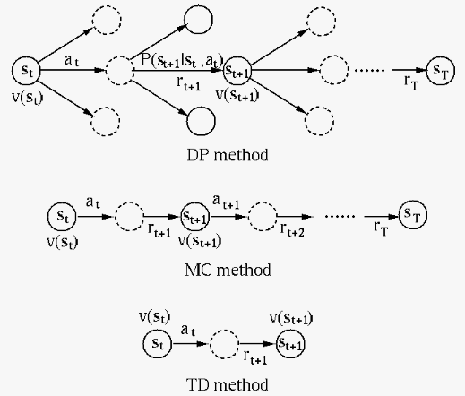
Here is the comparison of the MC and TD methods in terms of their pros and cons:

• The MC method estimates the state value $v_\pi(s_t)$, the expected return, by the true return $G_t$ obtained at the end of the episode, i.e., the estimated value is updated once every episode;

  The TD method estimates $v_\pi(s_t)$ as the sum of the immediate reward $r_{t+1}$ and the estimated state value at the next state $v_\pi(s')$, i.e., it is a bootstrap method, and the estimated value is updated at every step of every spisode.

• MC can only learn episodic (terminating) environments with complete episodes; while TD can learn continuing (non-terminating) environent of incomplete episodes.

• MC estimates $v_\pi(s_t)$ is based on sample returns $G_t$, and it is unbiased, while TD uses the bootstrap approach to find the TD target based on sample data that are not necessarily i.i.d., and it is more sensitive to the initial guess of the value functions, it is more biased.

• MC is based on the sample returns $G_t$ affected by many random events (state transitions, actions, and rewards), and in particular the first-visit version of the MC method only makes use of the sample data from the first visit of a state, it does not use the available data efficiently and it has high variance, while on the other hand the TD method is based on only one random variable, the estimated return, and it makes more frequent and efficient use of the sample data, it has lower variance.

• In the MC method, especially the first-visit version of it, the estimated value functions is unbiased; on the other hand, as the TD method is based on the bootstrap strategy and relies more strongly on the initial guess of the value functions being estimated, it tends to be more biased.

Here is a summary of the dynamic programming (DP) method for model-based planning, and the Monte-Carlo (MC) and time difference (TD) methods for model-free control: