TD($\lambda$) Algorithm

The MC and TD methods considered previously can be unified by the n-step TD($\lambda$) method that spans a spectrum of which the MC and TD methods are two special cases at the opposite extremes.

Recall that both MC and TD algorithms updates iteratively the value functions being estimated and the policy being improved based on Eq. (49), but they estimate the target $G_t$ in the equation differently. In an MC algorithm, the target is the actual return $G_t=r_{t+1}+\gamma r_{t+2}+\cdots+\gamma^{T-t-1} r_T$, the sum of discounted rewards of all future steps upto the terminal state $s_T$, available only at the end of each episode. On the other hand, in a TD algorithm, the target is $G_t=r_{t+1}+\gamma v_\pi(s){t+1})$ the sum of the immeidate reward $r_{t+1}$ available at each step of the episode, and the discounted value of the next state, based on bootstrapping. We therefore see that an MC algorithm updates the value functions and policy once every episode, while a TD algorithm updates once every step in the spisode.

As a trade-off between the MC and TD methods, the n-step TD algorithm can be considered a generalization of the TD method, where the target in Eq. (49) is an n-step return, the sum of the discounted rewards in the $n$ subsequent states and the discounted value function at the following state $s_{t+n}$ with $1\le n<\infty$:

$$G_{t:t+n}=r_{t+1}+\gamma r_{t+2}+\cdots+\gamma^{n-1} r_{t+n} +\gamma^n v_\pi(s_{t+n})$$ (57)

Specially, when

• $n=1$: the 1-step return is the sum of the immediate reward and the estimated value of the next state, the same as the TD target in the TD method:

  $$G_{t:t+1}=r_{t+1}+\gamma v(s_{t+1})$$ (58)

• $n=T-t$: the n-step return is the sum of the discounted rewards from all future states upto the terminal state at the end of the episode, i.e., it is the return $r_t$ defined in Eq. (7), the same as in the MC method:

  $$G_{t:t+n}=r_{t+1}+\gamma r_{t+2}+\gamma^2 r_{t+3} +\cdots +\gamma^{T-t-1}r_T+v_\pi(s_{t+n})=G_t$$ (59)

  where the value function of the terminal state $v_\pi(s_{t+n})=v_\pi(s_T)=0$ is zero.

• $T-t<n<\infty$: All states $s_n$ beyond the terminal state $s_T$ with $n>T-t$ remain the same as the terminal state with value $v(s_T)=0$ and return $G_t$, same as in the MC method.

We see that all these n-step returns form a spectrum with the MC and TD methods at the two ends.

Based on these n-step returns of different $n$ values, the n-step TD algorithm can be further generalized to a more computationally advantageous and therefore more useful algorithm called TD($\lambda$), by which the MC and TD algorithms are again unified as two special cases at the opposite ends of a spectrum.

We first define the $\lambda$-return $G_t^\lambda$ as the weighted average of all n-step returns for $n=1,2,\cdots,\infty$:

$$G_t^\lambda=(1-\lambda)\sum_{n=1}^\infty \lambda^{n-1}G_{t:t+n}$$ (60)

where $0\le\lambda<1$. Note that the weights decay exponentially, and they are normalized due to the coefficient $1-\lambda$:

$$(1-\lambda)\sum_{n=1}^\infty\lambda^{n-1} =(1-\lambda)\sum_{n=0}^\infty\lambda^n =\frac{1-\lambda}{1-\lambda}=1$$ (61)

The $\lambda$-return $G_t^\lambda$ defined above can be expressed in two summations, the sum of the first $T-t-1$ n-step returns $G_{t:t+1},\cdots,G_{t:t+T-1}$, and the sum of all subsequent n-step returns $G_{t:T}=\cdots=G_{t:\infty}=G_t$:

$$G_t^\lambda = (1-\lambda)\sum_{n=1}^{T-t-1} \lambda^{n-1}G_{t:t+n} +(1-\lambda)\sum_{n=T-t}^\infty \lambda^{n-1} G_t$$

$$= (1-\lambda)\sum_{n=1}^{T-t-1} \lambda^{n-1}G_{t:t+n} +\lambda^{T-t-1} G_t,\;\;\;\;\;\;\;(0\le t\le T)$$ (62)

where the coefficient of $G_t$ in the second term is the sum of coefficients in the second summation:

$$(1-\lambda)\sum_{n=T-t}^\infty \lambda^{n-1} =(1-\lambda) \sum_{m=0}^\infty\lambda^m \lambda^{T-t-1} =\lambda^{T-t-1}$$ (63)

where $m=n-T+t$. We see that in Eq. (62) all n-step returns $G_{t:t+n}$ are weighted by exponentially decaying coefficient $\lambda^{n-1}$, except the true return $G_t$ which is weighted by $\lambda^{T-t-1}$.

Again consider two special cases:

• $\lambda=0$: all terms in Eq. (62) are zero, except the first one with $n=1$:

  $$G_t^{\lambda=0}=\lambda^{n-1} G_{t:t+n}\bigg\vert _{n=1}=0^0\,G_{t:t+1} =r_{t+1}+\gamma v(s_{t+1})$$ (64)

  This is simply the TD target, i.e., TD(0) is the TD method.
• $\lambda=1$: the first summation is zero and

  $$G_t^{\lambda=1}=G_t$$ (65)

  i.e., TD(1) is the MC method.

We therefore see that TD($\lambda$) is a general algorithm of which the two special cases TD(0) and TD(1) are respectively the TD and MC methods.

In Eq. (62), $G_t^\lambda$ is calulated as the weighted sum of all n-step returns $G_{t:t+n}$ upto the last one $G_t$ available at the end of the episode. This summation can be truncated to include fewer terms before reaching the terminal state at the end of the episode:

$$G_{t:h}^\lambda =(1-\lambda)\sum_{n=1}^{h-t-1} \lambda^{n-1}G_{t:t+n} +\lambda^{h-t-1} G_{t:h},\;\;\;\;\;\;\;\;(0\le t<h\le T)$$ (66)

Specially when $h=T$, $G_{t:h}^\lambda=G_t^\lambda$ same as before, and when $h=t+1$, $G_{t:h}^\lambda=G_{t:t+1}=r_{t+1}+\gamma v(s_{t+1})$, same as the TD target.

Based on $\lambda$-return, the iterative update of the value function $v_\pi(s_t)$ in Eq. (52) can be modified to:

$$v_\pi(s_t)=v_\pi(s_t)+\alpha(G_t^\lambda-v_\pi(s_t)) =v_\pi(s_t)+\alpha\delta_t$$ (67)

where

$$\delta_t=G_t^\lambda-v_\pi(s_t)$$ (68)

This iteration is called the forward view of TD($\lambda$), which is similar to the MC method, as they are based on either $G_t$ or $G_t^\lambda$, available only at the end of each episode.

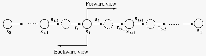
An alternative method is the backward view of TD($\lambda$), which can be shown to be equivalent to the forward-view of TD($\lambda$), but it is similar to the TD(0) method, as they are both based on the immediate reward $r_{t+1}$ available at each time step of the episode, and therefore more computationally convenient.

Specifically, the backward view of TD($\lambda$) is based the eligibility trace $e_t(s)$ for each of the states, which decays exponentially upon each state transition

$$e_t(s)=\gamma\lambda e_{t-1}(s)\;\;\;\;\;(\forall s\in S)$$ (69)

but is boosted by an increment $1$ to become $e_t(s)=e_t(s)+1$ if $s=s_t$ is currently visited.

Now the iterative update of the estimated value function in Eq. (52) is modified so that all states, instead of only the one currently visited, are updated, but to different extents based on $e_t(s)$:

$$v_\pi(s)=v_\pi(s)+\alpha\delta_te_t(s),\;\;\;\;\;\;\; \forall s\in S$$ (70)

where the TD error $\delta_t$ is the same as in TD(0), given in Eq. (53):

$$\delta_t=r_{t+1}+\gamma v_\pi(s_{t+1})-v_\pi(s)$$ (71)

The eligibility trace $e_t(s)$ as defined above is motivated by the frequency and recency of the visites to each state. If a state $s$ has been more frequently and recently visited compared to others, its $e_t(s)$ is greater than others and its value function $v_\pi(s)$ will be updated by a greater increment than others.

Here is the pseudo code for the backward view of the TD($\lambda$) methd for policy evaluation:

Input: policy $\pi$ to be evaluated

Initialize: $v(s)=0\;\;\forall s\in S$

loop (for each episode)

$s=s_0$

$e(s)=0,\;\forall s\in S$

while $s$ is not terminal (for each step)

take action $a$ based on $\pi(a\vert s)$, get reward $r$ and next state $s'$

$\delta=r+\gamma v(s')-v(s)$

$e(s)=e(s)+1$

for all $s$

$v(s)=v(s)+\alpha\delta e(s)$

$e(s)=\gamma\lambda e(s)$

$s=s'$

Note that values at all states are updated, but to different extents depending on $e(s)$, different from the TD algorithm where only the value at the state currently visited is updated.

Again consider two special cases:

• $\lambda=0$, $e(s)=0$ for all states except the current $s$ being visited, i.e., TD($\lambda$) becomes TD(0), the same as the TD method.
• $\lambda=1$, then $e(s)$ is scaled down by a factor $\gamma<1$ for all states except the current $s$ being visited, i.e., TD($\lambda$) becomes TD(1), the same as the MC method. However, different from the MC method that updates the value function $v(s)$ at the end of each spisode, here $v(s)$ is still updated at every step of the episode due to the backward view of the method.

This backward view of the TD($\lambda$) method can be applied to model-free control when the state value function is replaced by the action value function. Corresponding to the SARSA and Q-learning algorithms based on TD(0) in the previous section, here are the two algorithms based on eligibility traces:

• SARSA($\lambda$) algorithm:

  Initialize: $q(s,a)=0,\;\forall (s,a)$, $\alpha\in(0,\;1]$, $\epsilon>0$, denote $\epsilon$-greedy policy $\pi(a\vert s)$ by $\pi$

  loop (for each episode)

  $s=s_0$

  $e(s,a)=0,\;\forall (s,a)$

  get action $a$ according to $\pi$ based on $q(s,a)$

  while $s$ is not terminal (for each step)

  $e(s,a)=e(s,a)+1$

  take action $a$, get reward $r$ and next state $s'$

  get action $a'$ according to $\pi$ based on $q(s',a)$

  $\delta=r+\gamma q(s',a')-q(s,a)$

  for all $(s,a)$

  $q(s,a)=q(s,a)+\alpha\delta\, e(s,a)$

  $e(s,a)=\gamma\lambda e(s,a)$

  $s=s',\;a=a'$

• Q($\lambda$) algorithem:

  Initialize: $q(s,a)=0,\;\forall (s,a)$, $\alpha\in(0,\;1]$, $\epsilon>0$, denote $\epsilon$-greedy policy $\pi(a\vert s)$ by $\pi$

  loop (for each episode)

  $s=s_0$

  $e(s,a)=0,\;\forall (s,a)$

  get action $a$ according to $\pi$ based on $q(s,a)$

  while $s$ is not terminal (for each step)

  $e(s,a)=e(s,a)+1$

  take action $a$, get reward $r$ and next state $s'$

  get action $a'$ according to $\pi$ based on $q(s',a)$

  $a^*=\argmax_b q(s',b)$

  $\delta=r+\gamma q(s',a^*)-q(s,a)$

  for all $(s,a)$

  $q(s,a)=q(s,a)+\alpha\delta\, e(s,a)$

  if $a'=a^*$ then $e(s,a)=\gamma\lambda e(s,a)$ else $e(s,a)=0$

  $s=s',\;a=a'$

Note that Q($\lambda$) algorithm is different from the SARSA($\lambda$) algorithm in two ways. First, the action value is updated based on the greedy action $a^*$, instead of the $a'$ by policy $\pi$; second, if the $\epsilon$-greedy policy $\pi$ happens to choose a random non-greedy action $a'\ne a^*$ with probability $\epsilon$ to explore rather than exploiting $a^*$, the eligibility traces of all states are reset to zero. There are other different versions of the algorithm which do not reset these traces.