Model-Based Planning

Given a complete MDP model in terms of $p(s',r\vert s,a)$ of the environment, the goal of model-based planning is to find the optimal policy $\pi^*$ that achieves the maximum value:

$$v^*(s)=\max_\pi v_\pi(s),\;\;\;\;\;\;\;\;\;\;\; \pi^*(s)=\argmax_\pi v_\pi(s)\ge \pi\;\;\;\;\;\;\forall\pi$$ (25)

based on the partial order that compares different policies according to the corresponding values:

$$\;\;\;\;\; v_{\pi_1}(s)\ge v_{\pi_2}(s)\ge \cdots v_{\pi_k}(s), \;\;\;\;\forall s\in S$$ If

$$\;\;\;\; \pi_1\ge\pi_2\ge\cdots\ge\pi_k$$ Then (26)

The problem of policy optimization can be addressed based on two subproblems: policy evaluation to measure how good a policy is, and policy improvement to get a better policy for higher values.

One way to solve this optimization problem is to use brute-force search to enumerate all $\vert A(s)\vert$ available policies at each of the $N=\vert S\vert$ states $s\in S$. If we assume the numbers of avilable actions in all states are the same for simplicity, i.e., $A(s_1)=\cdots=A(s_N)=A$, then the computational complexity of this method is $O(\vert A\vert^{\vert S\vert})$, likely to be too high for such a brute-force search to be practical if $N$ is large.

A more efficient and therefore more practical way to optimize the policy is to do it iteratively. Consider a simpler task of improving upon an existing deterministic policy $\pi$ at a single transition step from the current state $s$ to a next state $s'$. Instead of taking the action $a=\pi(s)$ dictated by the policy, we can improve it by taking the greedy action that maximizes the action value function in Eq. (22), while subsequent steps still follow the old policy $\pi$. Now we get a new policy:

$$\pi'(s)=\argmax_a q_\pi(s,a) =\argmax_a \left[ r(s,a)+\gamma \sum_{s'} P(s'\vert s,a) v_\pi(s')\right]$$ (27)

so that the action value is higher than that of the old one:

$$q_\pi(s,\pi'(s))=\max_a q_\pi(s,a) =\max_a \left[ r(s,a)+\gamma \sum_{s'} P(s'\vert s,a) v_\pi(s')\right] \ge q_\pi(s,\pi(s))=v_\pi(s)$$ (28)

where the last equality is due to Eq. (24) for a deterministic policy.

While it is obvious that this greedy method will result in a higher return for the single state transition from $s$ to $s'$, we can further prove the following policy improvement theorem stating that following this greedy method in all subsequent states, we will get a new policy $\pi'$ that achieves higher values than the those of the old one $\pi$ at all states:

$$v_{\pi'}(s)\ge v_\pi(s),\;\;\;\;\;\;\;\forall s\in S$$ (29)

The proof is by recursively applying the greedy method to replace the old policy $\pi(s)$ by the new one $\pi'(s)$ for a higher value for each of the subsequent steps one at a time:

$$v_\pi(s) \le q_\pi(s,\pi'(s)) =\max_a q_\pi(s,a) =\max_a\left[ r(s,a)+\gamma \sum_{s'} P(s'\vert s,a) v_\pi(s')\right]$$

$$= r(s,\pi'(s))+\gamma \sum_{s'} P(s'\vert s,\pi'(s)) v_\pi(s')$$

$$\le r(s,\pi'(s))+\gamma \sum_{s'} P(s'\vert s,\pi'(s)) \max_{a'} q_\pi(s',a')$$

$$= r(s,\pi'(s))+\gamma \sum_{s'} P(s'\vert s,\pi'(s)) \left[ r(s',\pi'(s))+\gamma \sum_{s''} P(s''\vert s',\pi'(s')) v_\pi(s'')\right]$$

$$= r(s,\pi'(s))+\gamma r(s',\pi'(s))+ \gamma \sum_{s'} P(s'\vert s,\pi'(s)) \left[ \gamma \sum_{s''} P(s''\vert s',\pi'(s')) v_\pi(s'')\right]$$

$$\le \cdots$$

$$= r(s,\pi'(s))+\gamma r(s',\pi'(s'))+\gamma^2 r(s'',\pi'(s'') + \cdots$$

$$= v_{\pi'}(s)$$ (30)

i.e., $\pi'(s)\ge\pi(s)$.

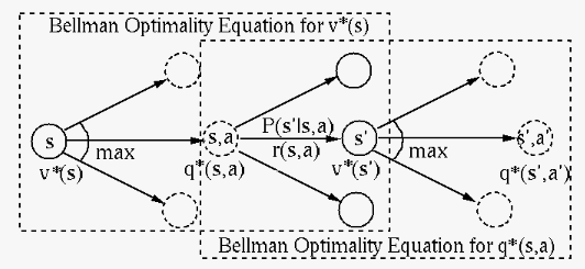
The optimal state value $v^*(s)$ and action value $q^*(s,a)$ can therefore be achieved by replacing the weighted average over all possible actions at each state ($s$ and $s'$) in the Bellman equations in Eqs. (21) and (22) by their maximum:

$$v^*(s)=\max_a q^*(s,a) =\max_a \left( r(s,a)+\gamma \sum_{s'} P(s'\vert s,a) v^*(s') \right)$$ (31)

and

$$q^*(s,a)=r(s,a)+\gamma \sum_{s'} P(s'\vert s,a) v^*(s') =r(s,a)+\gamma \sum_{s'} P(s'\vert s,a) \max_{a'} q^*(s',a')$$ (32)

Eqs. (31) and (32) are the Bellman optimality equations, which should hold for all $N$ states in $S=\{s_1,\cdots,s_N\}$ and can be written in vector form:

$${\bf v}^*=\max_a\left({\bf r}_a +\gamma{\bf P}_a{\bf v}^*\right)$$ (33)

where

$${\bf v}^*=\left[\begin{array} {c}v^*(s_1)\\ \vdots\\ v^*(s_N)\end... ...s & \vdots \\ P(s_1\vert s_N,a) & \cdots & P(s_N\vert s_N,a)\end{array}\right]$$ (34)

This nonlinear equation system can be solved iteratively to for ${\bf v}^*$:

$${\bf v}^*_{n+1} =\max_a\left({\bf r}_a +\gamma{\bf P}_a{\bf v}^*_n \right)=B({\bf v}_n)$$ (35)

This iteration is to be used for policy evaluation in the algorithm value iteration below for finding the optimal policy. This iteration will converge as function $B({\bf v})$ is a contraction mapping with $\gamma<1$:

$$\vert\vert B({\bf v}_i)-B({\bf v}_j)\vert\vert = \vert\vert\max_{a_i}\left({\bf r}_{a_i}+\gamma{\bf P}_{a_i}{\bf v... ...) -\max_{a_j}\left({\bf r}_{a_j}+\gamma{\bf P}_{a_j}{\bf v}_j \right)\vert\vert$$

$$\le \vert\vert\max_{a_i} \left({\bf r}_{a_i}+\gamma {\bf P}_{a_i}{\bf v}_i -{\bf r}_{a_i}-\gamma{\bf P}_{a_i}{\bf v}_j \right)\vert\vert$$

$$= \max_{a_i}\gamma\vert\vert{\bf P}_{a_i} ({\bf v}_i-{\bf v}_j)\ver... ...amma\vert\vert{\bf P}_{a_i}\vert\vert\; \vert\vert{\bf v}_i-{\bf v}_j\vert\vert$$

$$= \gamma\vert\vert{\bf v}_i-{\bf v}_j\vert\vert<\vert\vert{\bf v}_i-{\bf v}_j\vert\vert$$ (36)

where $\vert\vert{\bf P}\vert\vert=\vert\vert{\bf P}\vert\vert _\infty=1$ is the p-norm ($p=\infty$) of a stochastic matrix, which is known to be 1.

Given the complete information of the MDP model in terms of $p(s',r\vert s,a)$, we can find the optimal policy $\pi^*$ using either policy iteration (PI) or value iteration (VI) based on the DP method.

• Policy Iteration

  Carry out the following two processes iteratively from some arbibrary initial policy $\pi$ until convergence when $\pi$ no longer changes:

  • Policy evaluation:

    Given a deterministic policy $\pi$, Eq. (21) becomes the Bellman equation in Eq. (24), a linear equation system of $N=\vert S\vert$ equations of $N$ unknowns $v_\pi(s_1),\cdots,v_\pi(s_N)$, which can be solved iteratively as in Eq. (12) to find values at all states:

    $v_{n+1}^\pi(s)=r(s,\pi(s))+\gamma\sum_{s'}P(s'\vert s,\pi(s)) v_n^\pi(s') \;\;\;\;\;\;\;\;\;\;\;\; \forall s\in S$

  • Policy improvement:

    Given $v_\pi(s)$ based on policy $\pi$, get a better policy $\pi'$ by the greedy method as in Eq. (27):

    $\pi'(s)=\argmax_a\left[ r(s,a) +\gamma\sum_{s'}P(s'\vert s,\pi(s)) v_\pi(s')\right] \;\;\;\;\;\;\;\;\forall s\in S$

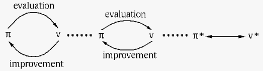
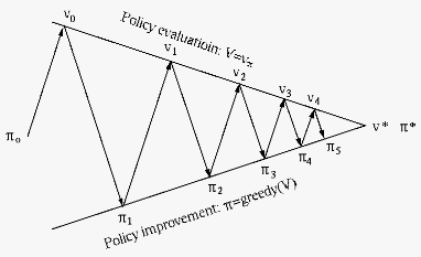
  We see that in each round of the policy iteration, two intertwined and interacting processes, the policy evaluation and policy improvement, are carried out alternatively, one depending on the other, and one completing before the other starts. The value functions $v_\pi(s)$ at all states are sysmeticaly evaluated before they are updated, and the policy $\pi(a\vert s)$ at all states is updated before it is evaluated. While these two processes chase each other as moving target iteratively and eventually converge to the optimal policy $\pi^*$ achieving the optimal value $v^*$. This approach is said to be synchronous, as shown here:

  $$\pi_o\stackrel{E}{\longrightarrow} v_{\pi_0}\stackrel{I}{\longrig... ...s \stackrel{I}{\longrightarrow}\pi^* \stackrel{E}{\longrightarrow}v_{\pi^*}=v^*$$ (37)

  The pseudo code for the algorithm is listed below:

  Initialize:

  $v(s)\in \mathbb{R},\;$   $\mbox{$v(s)=0$\ if $s$\ is terminal node}$$, \;\pi(s)\in A(s),\;\;\forall s\in S$;

  Set tolerence $tol$ (small positive value);

  repeat

  Policy Evaluation (find $v(s)\;\;\forall s\in S$):

  repeat

  $\delta=0$

  for $\forall s\in S$:

  $v'(s)=r(s,\pi(s))+\gamma\sum_{s'}P(s'\vert s,\pi(s))v(s')$

  $\delta=\max(\delta,\vert v(s)-v'(s)\vert)$

  until $\delta<tol$

  Ploicy Improvement (by taking greedy action):

  $Done=T$

  for each $s\in S$

  $\pi'(s)=\argmax_a\left[r(s,a)+\gamma\sum_{s'} P(s'\vert s,\pi(s)) v(s')\right]$

  if $\pi'(s)\ne\pi(s),\;\;Done=F$

  end for

  until $done$

• Value Iteration:

  One drawback of the policy iteration method is the high computational complexity of the inner iteration for policy evaluation inside the outer iteration for policy evaluation. To speed up this process, we could terminate the inner iteration early before convergence. In the extreme case, we simply combine policy evaluation and improvement into a single step, resulting in the following value iteration contains two steps:

  • Find the optimal values:

    Based on some initial value $v_0(s)$, solve the Bellman optimality equation in Eq. (31) by iteration in Eq. (35):

    $$v_{n+1}(s)=\max_a\left[r(s,a)+\gamma\sum_{s'} P(s'\vert s,a)v_n(s')\right] \;\;\;\;\;\;\forall s\in S$$ (38)

  • Find the optimal policy:

    Find $\pi^*(s)$ that maximizes $v^*(s)$:

    $$\pi^*(s)=\argmax_a\left[r(s,a)+\gamma \sum_{s'}P(s'\vert s,a)v_n(s')\right] \;\;\;\;\;\;\forall s\in S$$ (39)

  Here is the pseudo code for the algorithm:

  Initialize: $v(s)=0\;\;\forall s\in S$

  repeat

  $\delta=0$;

  for each $s\in S$

  $v'(s)=\max_a\left[r(s,a)+\gamma\sum_{s'}P(s'\vert s,a)v(s')\right]$

  $\delta=\max(\delta,\vert v'(s)-v(s)\vert)$

  $v(s)=v'(s)$

  end for

  until $\delta<tol$

  $\pi^*(s)=\argmax_a\left[r(s,a)+\gamma\sum_{s'}P(s'\vert s,a)v(s')\right]$

In the PI method considered above, the value functions at all states are evaluated before the policy is updated for all states, as illustrated below:

This synchronous policy iteration can be modified so that the values at some or even one of the states are evaluated in-place before other state values are updated, and the policy at some or even one of the states are updated in-place before that at other states, resulting in an asynchronous method called general policy iteration (GPI), to be discussed in detail in the next sections on model-free control.