Markov Decision Process

Markov decision process (MDP) is the mathematical framework for reinforcement learning. To understand MDP, we first consider the basice concept of Markov process or Markov chain, a stochastic model of a system that can be characterized by a set of states $S=\{s_1,\cdots,s_N\}$ of size $\vert S\vert=N$ (cardinality of $S$). The dynamics of the system in terms of its state transition is modeled by the transition probability $P_{ij}=P(s_j\vert s_i)$ from the current state $s_t=s_i$ to the next state $s_{t+1}=s_j$ with $i,j=1,\cdots,N$. The system is assumed to be memoryless, i.e., its future is independent of the past history $h_t=\{s_t,s_{t-1},\cdots,s_0\}$, given the present $s_t$:

$$P(s_{t+1}\vert h_t)=P(s_{t+1}\vert s_t,s_{t-1},\cdots,s_0)$$ (1)

For example, if the state of a helicopter is described by its linear and angular position and velocity based on which its future position and velocity can be completely determined, then it can be modeled by a Markov process; but if the state is only described by its position, then its position in the past is needed for determining its future (e.g., to find its velocity), and it is not a Markov process.

All transition probabilities can be organized as an $N\times N$ state transition matrix:

$${\bf P}=\left[\begin{array}{ccc} P_{11} & \cdots & P_{1N}\\ \vdots & \ddots & \vdots \\ P_{N1} & \cdots & P_{NN}\end{array}\right]$$ (2)

As the transition probabilities from any current state $s_i$ to the $N$ possible next states $s_1,\cdots,s_N$ have to sum up to 1, we have

$$\sum_{j=1}^N P_{ij}=\sum_{j=1}^N P(s_j\vert s_i)=1, \;\;\;\;\;\;\;(i=1,\cdots,N)$$ (3)

Any matrix satisfying this property is called a stochastic matrix.

In the following, our discussion is mostly concentrated on the the general transition from the current state $s_t=s$ to the next state $s_{t+1}=s'$ with transition probability $P(s_{t+1}=s'\vert s_t=s)=P_{s s'}$.

Example Weather in Los Angeles:

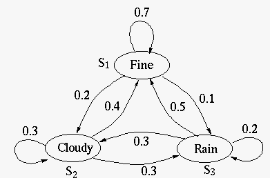
$${\bf P}=\left[\begin{array}{ccc} 0.7 & 0.2 & 0.1 \\ 0.4 & 0.3 & 0.3 \\ 0.5 & 0.2 & 0.3 \end{array}\right]$$ (4)

We next consider a Markov reward process (MRP), represented by a tuple $\langle S, P, R, \gamma\rangle$ of four elements for the states, state transition probabilities, rewards, and the discount factor. Here the reward $R$ can be considered as a feedback signal to the agent at each time step of the sequence of state transitions, indicating how well it is doing with respect to the overall task. The reward can be negative, as a penalty, for situations to be avoided. The performance of the agent is measured by the sum of rewards accumulated over all time steps of the Markov process, weighted by the discount factor $\gamma \in[0,\;1]$ that discounts future rewards. If $\gamma$ is close to 0, then the immediate reward is emphasized (short-sighted or greedy), but if $\gamma$ is close to 1, then rewards in the future steps will be almost as valuable as immediate ones (far-sighted).

The sequence of state transitions of an MRP from an initial state $s_0$ to a terminal state $s_T$ is called an episode, and the number of time steps $T$ is called horizon, which can be either finite or infinite.

Both the reward $r$ and the next state $s'$ resulting from arriving at the current state $s$ are considered as random variables with joint probability $p(s',r\vert s)=P(s_{t+1}=s',r_{t+1}=r\vert s_t=s)$, based on which both the state transition probability and state reward probability can be found by marginalization:

$$p(s'\vert s)=P(s_{t+1}=s'\vert s_t=s)=\sum_{r\in R} p(s',r\vert s), \;\;\;\;\;\;\;\;\;\; P(r\vert s)=\sum_{s'\in S} p(s',r\vert s)$$ (5)

Note that conventionally the reward $r$ received after arriving at state $s_t$ is denoted by $r_{t+1}$, instead of $r_t$. The index $s'\in S$ for the summation over all states will be abbreviated to $s'$ in the subsequent discussion. The expectation of the reward at $s$ is

$$r(s)=E[ r_{r+1}\vert s_t=s]=\sum_r r P(r\vert s) =\sum_r r \sum_{s'} P(s',r\vert s)$$ (6)

We define the return $G_t$ at each step $s=s_t$ as the accumlate reward, the sum of the immediate reward after arriving at the current state $s=s_t$ and all delayed rewards in the future states upto a terminal state $s_T$ with reward $r_T$ at the end of the episode, discounted by $\gamma$:

$$G_t=r_{t+1}+\gamma r_{t+2}+\gamma^2 r_{t+3}+\cdots+ \gamma^{T-t-1} r_T =\sum_{k=0}^{T-t-1} \gamma^k r_{t+k+1}$$ (7)

We further define the state value function $v(s)$ at state $s=s_t$ as the expectation of the return, which can be further expressed recursively in terms of the values $v(s')$ of all possible next states $s'=s_{t+1}$:

$$v(s) = E[ \;G_t\vert s_t=s \;] =E [r_{t+1}+\gamma r_{t+2}+\gamma^2 r_{t+3} +\cdots \vert s_t=s]$$

$$= E [r_{t+1}+\gamma (r_{t+2}+\gamma r_{t+3} +\cdots) \vert s_t=s]$$

$$= E[r_{t+1}\vert s=s_t]+\gamma E[ G_{t+1} \vert s_{t+1}=s',\,s_t=s]$$

$$= r(s)+\gamma \sum_{s'} P(s'\vert s) v(s')$$ (8)

where $r(s)$ is given in Eq. (6). The value of a terminal state $s_T$ at the end of an episode is zero, as there will be no next state and thereby no more future reward.

This equation is called the Bellman equation, by which the value $v(s)$ at current state $s$ is expressed recursively in terms of the immediate reward $r(s)$ and the values $v(s')$ of all possible next states, without explicitely invoking all future rewards. Based on this bootstrap idea of the Bellman equation, a multi-step MRP problem can be expressed recursively as a subproblem concerning only a single state transition from $s$ to $s'$, as a backward induction to find current state value from all future ones. For this reason, the Bellman equation plays an essential role in future discussion of some important algorithms in reinforcement learning.

The Bellman equation in Eq. (8) holds for all states $s_1,\cdots,s_N$, and the resulting $N$ equations can be expressed in vector form as:

$${\bf v} = \left[\begin{array}{c}v(s_1)\\ \vdots\\ v(s_N)\end{array}\right] ... ...rray}\right] \left[\begin{array}{c} v(s_1)\\ \vdots\\ v(s_N)\end{array} \right]$$

$$= {\bf r}+\gamma {\bf P}{\bf v}$$ (9)

where ${\bf P}$ is called the stochastic matrix. Solving this linear equation system of size $N$ we find

$${\bf v}=({\bf I}-\gamma{\bf P})^{-1} {\bf r}$$ (10)

Such a solution exists as matrix ${\bf I}-\gamma{\bf P}$ is invertible. This can be shown by noting that all eigenvalues of the stochastic matrix ${\bf P}$ are not greater than 1: $\vert\lambda\vert \le 1$ (see here), and all eigenvalues of $\gamma{\bf P}$ are smaller than 1: $\gamma\lambda<1$, i.e., the eigenvalue of ${\bf I}-\gamma{\bf P}$ is greater than zero: $1-\gamma\lambda>0$. Consequently the determinant $\det({\bf I}-\gamma{\bf P})$ of this coefficient matrix, as the product of all its nonzero eigenvalues, is non-zero and therefore matrix $\det({\bf I}-\gamma{\bf P})$ is invertible.

Alternatively, the Bellman equation in Eq. (8) can also be solved iteratively by the general method of dynamic programming (DP), which solves a multi-stage planning problem by a backward induction and find the value function recursively. We first rewrite the Bellman equation as

$${\bf v}={\bf r}+\gamma{\bf Pv}=B({\bf v})$$ (11)

where $B({\bf v})={\bf r}+\gamma{\bf Pv}$ is defined as a vector-valued function (an operator) applied to the vector argument ${\bf v}$. Now the Bellman equation can be solved iteratively from an arbitrary initial value, such as ${\bf v}_0={\bf0}$:

$${\bf v}_{n+1}=B({\bf v}_n)={\bf r}+\gamma{\bf Pv}_n$$ (12)

This iteration will always converge to the root of the equation, the fixed point of function $B({\bf v})$, as it is a contraction mapping satisfying

$$\vert\vert B({\bf v}_i)-B({\bf v}_j)\vert\vert = \vert\vert{\bf r}+\gamma{\bf Pv}_i -\left({\bf r}+\gamma{\bf Pv}_j \right)\vert\vert =\gamma\vert\vert{\bf P}({\bf v}_i-{\bf v}_j)\vert\vert$$

$$\le \gamma\vert\vert{\bf P}\vert\vert\; \vert\vert{\bf v}_i-{\bf v}_j... ...\vert\vert{\bf v}_i-{\bf v}_j\vert\vert<\vert\vert{\bf v}_i-{\bf v}_j\vert\vert$$ (13)

That $B({\bf v})$ is a contraction can also be proven by showing the norm of its Jacobian matrix, its derivative with respect to its vector argument ${\bf v}$, is smaller than 1. We first find the Jacobian matrix

$${\bf J}_B=\frac{d}{d{\bf v}}B({\bf v}) =\frac{d}{d{\bf v}} ( {\bf r}+\gamma{\bf Bv} )=\gamma{\bf P}$$ (14)

and then find its p-norm with $p=\infty$ (equivalent to $p=1,\;2$), the maximum absolute row sum:

$$\vert\vert{\bf J}_B\vert\vert _{p=\infty}=\vert\vert\gamma{\bf P}... ...t\vert _\infty =\gamma \max_{1\le i\le N}\sum_{j=1}^N\vert P_{ij}\vert=\gamma<1$$ (15)

The last equality is due to Eq. (3), i.e., $\vert\vert{\bf P}\vert\vert _\infty=1$.

In summary, the Bellman equation in Eq. (8) can be solved by either of the two methods in Eqs. (10) and (12), so long as $\gamma<1$. When the size of state space $\vert S\vert=N$ is large, the complexity $O(N^3)$ is too high then the iterative method may be more efficient.

Based on the definition of MRP, we further define Markov decision process (MDP) as an MRP with certain decision-making rule called policy, denoted by $\pi$, following the policy the agent takes one of the actions $a\in A(s)$ available at each state $s$ to control the state transition of the process. An MDP can therefore be described by a tuple $<S,P,R,A,\gamma>$, of which $A$ is the set of all actions. The policy $\pi$ can be either stochastic denoted by $\pi(a\vert s)=P(a_t=a\vert s_t=s)$ as the conditional probability of taking action $a$ in state $s$, or deterministic denoted by $a=\pi(s)$. A policy is soft if any of the actions available at a state is possible to be taken, i.e., $\pi(a\vert s)>0$ for all $a\in A(s)$ and all $s\in S$. In particular, a policy is $\epsilon$-soft if $\pi(a\vert s)\ge\epsilon/\vert A(s)\vert$ for some small value of $\epsilon$.

As there are $\vert A(s_n)\vert$ possible actions to take in state $s_n\in S$, the total number of policies is $\vert A(s_1)\vert \cdots \vert A(s_N)\vert=\Pi_{n=1}^N \vert A(s_n)\vert$. If the number of available actions $\vert A\vert$ is the same for all $\vert S\vert$ states, then the total number of policies is $\vert A\vert^{\vert S\vert}$.

Following a given policy from an initial state $s_0$ will result a sequence of state transitions called a trajectory of the episode:

$$s_0\stackrel{a_0}{\longrightarrow}s_1 \stackrel{a_1}{\longrightarrow}s_2 \stackrel{a_2}{\longrightarrow}s_3 \cdots s_T$$ (16)

of which the state visited at the t-th step denoted by $s_t$ can be any of the $N$ states in $S=\{s_1,\cdots,s_N\}$ of the MDP, not to be confused with the t-th state in $S$. Note that in an episode some of the states in $S$ may be visited multiple times, while some others may never be visited. Also note that due to the random nature of the MDP, following the same policy may not result in the same trajectory.

Along the trajectory of an episode, an accumulation of discounted rewards from all states visited will be received. Our goal is to find the optimal policy as a sequence of actions $a_0,\,a_1,a_2,\cdots$ for a given MDP model of the environment in terms of its state transition dynamics and rewards, so that the value $v(s_0)$ at the start state $s_0$, the expectation of the sum of all discounted future rewards, is maximized. This optimization problem can be solved by the method of dynamic programming, and such a process is called planning.

In an MDP, both the next state $s'$ and reward $r$ are assumed to be random variables with joint probability $p(s',r\vert s,a)=P(s_{t+1}=s',r_{t+1}=r\vert s_t=s,\,a_t=a)$ conditioned on the action $a$ and the previous state $s$. The state transition probability becomes

$$p(s'\vert s,a)=P(s_{t+1}=s'\vert s_t=s, a_t=a)=\sum_{r\in R} p(s',r\vert s,a)$$ (17)

and the expected reward $r$ received after arriving at the current is

$$r(s,a)=E[ r_{t+1} \vert s_t=s, a_t=a ] =\sum_r r\; p(r\vert s,a)=\sum_r r \sum_{s'} p(s',r\vert s,a)$$ (18)

Following a specific random policy $\pi(a\vert s)$, the agent takes an action $a\in A(s)$ to transit from the current state $s_t=s$ to the next state $s_{t+1}=s'$ with probability

$$p_\pi(s'\vert s)=P(s_{t+1}=s'\vert s_t=s) =\sum_{a\in A(s)} \pi(a\vert s)\; p(s'\vert s,a)$$ (19)

satisfying $\sum_{s'} P_\pi(s'\vert s) = 1$ and the reward in state $s$:

$$r_\pi(s)=E_\pi[ r_{t+1}\vert s_t=s]=\sum_{a\in A(s)}\pi(a\vert s)\;r(s,a)$$ (20)

where $E_\pi$ denotes the expectation with respect to a certain policy $\pi(a\vert s)$. The summation over all available actions $a\in A(s)$ in state $s$ will be abbreviated to $a$ in the following.

We further define two important functions with respect to a given policy $\pi$ of an MDP:

• The state value function $v_\pi(s)$ is the expected return at each state $s$ of the MDP while following policy $\pi$, similar to the value function of an MRP as $v(s)$ in Eq. (8), but now treated as a function of action $a$ as well as state $s$:
  

  $$v_\pi(s) = E_\pi [ G_t \vert s_t=s]$$

  $$= \sum_a\pi(a\vert s)\left(r(s,a) +\gamma\sum_{s'} P(s'\vert s,a)\;v_\pi(s') \right)$$

  $$= \sum_a \pi(a\vert s)\;q_\pi(s,a)$$ (21)

  
  where $q_\pi(s,a)$ is defined below.
• The state-action value function $q_\pi(s,a)$ is the expected return of taking a specific action $a$ (irrelevant to policy $\pi$) in state $s$, and then following $\pi$ in all subsequent states:
  

  $$q_\pi(s,a) = E_\pi\left[ G_t\vert s_t=s, a_t=a \right]$$

  $$= r(s,a)+\gamma\sum_{s'} P(s'\vert s,a)\;v_\pi(s')$$

  $$= r(s,a)+\gamma\sum_{s'} P(s'\vert s,a)\;\sum_{a'} \pi(a'\vert s')\;q_\pi(s',a') )$$ (22)

  
  where $v_\pi(s')$ is recursively represented as a weighted sum of $q_\pi(s',a')$ based on Eq. (21).

The state-action value $q_\pi(s,a)$ plays a more important role than $v_\pi(s)$ as it allows the freedom of taking any action independent of a given policy $\pi$, thereby allowing the opportunity to improve an existing policy, e.g., by taking a greedy action to maximize the value $q_\pi(s,a)$. The state-action value function $q_\pi(s,a)$ is often abbreviated as the action value ore Q-value for convenience in future discussions.

As a function of the state-action pair $(s,a)$, the state action value $q_\pi(s,a)$ can be represented as a table of $\vert S\vert$ rows each for one of the states $s$, and $\vert A\vert$ columns each for one of the actions $a$. The Q-value for each state-action pair stored in the table can be updated iteratively by various algorithms for learning the Q-values.

In particular, if the policy is deterministic with $\pi(a\vert s)=1$ and $a=\pi(s)$, then we have

$$P_\pi(s'\vert s)=P(s'\vert s,a),\;\;\;\;\;\;\;\;r_\pi(s)=r(s,a)$$ (23)

and the Bellman equations in Eqs. (21) and (22) become the same:

$$v_\pi(s)=r(s,a)+\gamma\sum_{s'} P(s'\vert s,a)\;v_\pi(s') =q_\pi(s,\pi(s))$$ (24)

same as the Bellman equation of an MRP in Eq. (8), and can be solved iteratively if $\gamma<1$, same as in Eq. (12).

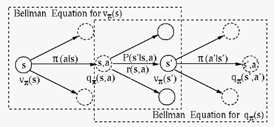
The figure above illustrates the Bellman equations in Eqs. (21) and (22), showing the bootstrapping of the state value function in the dashed box on the left, and that of the action value function in dashed box on the right. Specifically here the word bootstrapping means the iterative method that updates the estimated value at a state $s$ based on the estimated value of the next state $s'$. After taking oen of the actions $a\in A(s)$ available in state $s$ based on policy $\pi(a\vert s)$, an immediate reward $r(s,a)$ is received. However, which state the MDP will transit into as the next state $s'$ is random depending on $P(s'\vert s,a)$ of the environment but independent of the policy. This uncertanty is represented graphically by a dashed circle called a chance node associated with the action value $q_\pi(s,a)$ as the sum of the immediate reward $r(s,a)$ and the expected value of the next state, the weighted average of values $v(s')$ of all possible state $s'\in S$.