First Order Systems

In the previously discussed method for AC circuit analysis, all voltages and currents are represented as phasors and all circuit components (R, C, and L) are represented by their impedences, so that we can solve the corresponding algebraic equations to get the steady state responses of the circuit to an AC voltage or current input. However, if we are also interested in the transient response of the circuit to an input which is turned on at time moment $t=0$, we need to solve the corresponding differential equations to find its complete solution as the sum of the homogeneous solution and its particular solution.

As a simple example, the RC circuit shown below is composed of a resistor $R$ and capacitor $C$ in series with an external voltage input $v(t)$, which is turned on at $t=0$, either by a switch or a step voltage $v(t)$. We also assume the initial condition that the voltage across $C$ is $v_C(0)=V_0$ at $t=0$. Any of the variables $v_R(t)$, $v_C(t)$, and $i(t)$ can be considered as the circuit's response to this input.

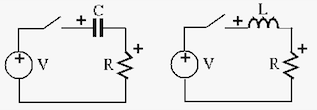
As shown in the figure, the polarity of $v_R$ is positive on top, and the polarities of $v_C$ is positive on the left.

• The RC circuit can be described by the KVL:

  $$v_R(t)+v_C(t)=R\;i(t)+v_C(t)=RC\frac{d}{dt} v_c(t)+v_c(t) =\tau \frac{d}{dt} v_C(t)+v_C(t)=v(t)$$ (68)

  where $\tau=RC$ is the time constant of the system with the dimension of time:

  $$[RC]=\frac{[V]}{[I]}\frac{[Q]}{[V]}=\frac{[Q]}{[I]}=[T]$$ (69)

• Similarly, for the RL circuit we have:

  $$v_R(t)+v_L(t)=R\; i(t)+L\frac{d}{dt} i(t)=v(t) \;\;\;\; \;\;\;\;\; \tau \frac{d}{dt} i(t)+i(t)=\frac{v(t)}{R}$$ (70)

  where $\tau=L/R$ is the time constant with the dimension of time:

  $$\frac{[L]}{[R]}=\frac{[V][T]}{[I]}\frac{1}{[R]}=\frac{[R][T]}{[R]}=[T]$$ (71)

In general, a first-order linear system with input $x(t)$ and output $y(t)$ can be described by a first-order linear-constant coefficient differential equation (LCCDE) in the canonic form:

$$\tau\frac{d}{dt}y(t)+y(t)=x(t)$$ (72)

in terms of a single parameter, the time constant $\tau$.

The solution of a DE represents the response (or output) of the circuit to both the external input and the initial state, and is composed of two parts:

• Homogeneous solution representing the natural response or transient response caused by the initial condition,
• Particular solutions representing the forced response or steady state response caused by the external input.