Next: Hierarchical (Tree) Classifiers Up: ch9 Previous: Multi-Class Classification
The naive Bayes (maximum likelihood) classification is based on a quadratic decision function and is therefore unable to classify data that are not quadratically separable. However, as shown below, the Bayes method can be reformulated so that all data points appear in the form of an inner product, and the kernel method can be used to map the original space into a higher dimensional space in which all groups can be separated even though they are not quadratically separable in the original space.
Consider a binary Bayes classifier by which any sample  is
classified into either of the two classes
is
classified into either of the two classes  and
and  depending on
whether is on the positive or negative side of the quadratic
decision surface (Eq. (22)):
depending on
whether is on the positive or negative side of the quadratic
decision surface (Eq. (22)):
 |
(172) |
 |
 |
 |
|
 |
|
 |
|
 |
|
 |
(173) |
 and
and
 are respectively the
covariance matrices of the samples in and ,
are respectively the
covariance matrices of the samples in and ,
 |
(174) |
 and
and  are their prior
probabilities. Specially if
are their prior
probabilities. Specially if
 and therefore
 , the quadratic decision surface becomes
a linear decision plane discribed by
, the quadratic decision surface becomes
a linear decision plane discribed by
![$\displaystyle f({\bf x})={\bf w}^T{\bf x}+w
=\left[{\bf\Sigma}^{-1}({\bf m}_+-{\bf m}_-)\right]^T{\bf x}+w=0$](img656.svg) |
(175) |
is classified into either of the two classes
depending on on which side of a threshold  its projection onto the
normal direction
its projection onto the
normal direction  of the decision plane lies.
As matrices  ,
,
 , and
, and
 are all symmetric, they can be written in the following
eigendecomposition
form:
are all symmetric, they can be written in the following
eigendecomposition
form:
 |
(176) |
 and
and
 . We can write vector
as:
. We can write vector
as:
 |
(177) |
can now be classified into either
of the two classes based on its decision function:
 |
|
 |
|
|
 |
||
|
 |
(178) |
 |
(179) |
 is defined as a function composed of all terms
in
is defined as a function composed of all terms
in
 except the last offset term
  , which is to replace
 in the original space. To find this , we first map all
training samples into a 1-D space
in the original space. To find this , we first map all
training samples into a 1-D space
 and sort them together with their corresponding labelings
 , and then search through all
  possible
ways to partition them into two groups indexed respectively by
possible
ways to partition them into two groups indexed respectively by
 and
and
 to find the optimal
  corresponding
to the maximum labeling consistency measured by
The middle point
corresponding
to the maximum labeling consistency measured by
The middle point
 between
  and
and  is used
as the optimal threshold to separate the training samples into two
classes in the 1-D space, i.e., the offset is
is used
as the optimal threshold to separate the training samples into two
classes in the 1-D space, i.e., the offset is
 .
Now the unlabeled point can be classified into either of
the two classes and :
.
Now the unlabeled point can be classified into either of
the two classes and :
 |
(182) |
In general, when all data points are kernel mapped to a higher
dimensional space, the two classes can be more easily separated,
even by a hyperplane based on the linear part of the decision
function without the second order term. This allows the assumption
that the two classes have the same covariance matrix so that
 and the second
order term is dropped. This is the justification for the following
two special cases:
and the second
order term is dropped. This is the justification for the following
two special cases:
and
by their average
 ,
then
and the decision function of any
becomes
,
then
and the decision function of any
becomes
 ,
,
 ,
,
 , and
, and
 .
This decision function can be converted to the following if the
kernel method is used:
.
This decision function can be converted to the following if the
kernel method is used:
 |
(184) |
 , then
the decision function above becomes
, then
the decision function above becomes
Note that if the kernel method is used to replace an inner product by
a kernel function
 ,
we need to map all data points to
,
we need to map all data points to
 in the higher dimensional space, instead of only mapping their means
 and
and
 , because the mapping of a sum
is not equal to the sum of the mapped points if the kernel is not linear:
, because the mapping of a sum
is not equal to the sum of the mapped points if the kernel is not linear:
 |
(187) |
The Matlab code for the essential part of the algorithm is listed
below. Given X and y for the data array composed of  training vectors
![${\bf X}=[{\bf x}_1,\cdots,{\bf x}_N]$](img9.svg) and their
corresponding labelings
and their
corresponding labelings
![${\bf y}=[y_1,\cdots,y_N]$](img702.svg) , the code carries
out the training and then classifies any unlabeled data point into
either of the two classes. Parameter
, the code carries
out the training and then classifies any unlabeled data point into
either of the two classes. Parameter type selects any one of
the three different versions of the algorithm, and the function
K(X,x) returns a 1-D array containing all kernel functions
 of the column vectors in
 and vector .
    X=getData;
    [m n]=size(X);
    X0=X(:,find(y>0));   n0=size(X0,2);     % separate C+ and C-
    X1=X(:,find(y<0));   n1=size(X1,2);
    m0=mean(X0,2);    C0=cov(X0');          % calculate mean and covariance
    m1=mean(X1,2);    C1=cov(X1');
    if type==1
        for i=1:n
            x(i)=sum(K(X0,X(:,i)))/n0-sum(K(X1,X(:,i)))/n1;
        end
    elseif type==2
        C=inv(C0+C1);   [V D]=eig(C);   U=(V*D^(1/2))';
        Z=U*X;  Z0=U*X0;   Z1=U*X1;
        for i=1:n
            x(i)=sum(K(Z0,Z(:,i)))/n0-sum(K(Z1,Z(:,i)))/n1;
        end
    elseif type==3
        C0=inv(C0);   C1=inv(C1);   W=-(C0-C1)/2;
        [V D]=eig(W);     U=(V*D^(1/2)).';    Z=U*X;
        [V0 D0]=eig(C0);  U0=(V0*D0^(1/2))';  Z0=U0*X;  Z00=U0*X0;
        [V1 D1]=eig(C1);  U1=(V1*D1^(1/2))';  Z1=U1*X;  Z11=U1*X1;
        for i=1:n
            x(i)=K(Z(:,i),Z(:,i))+sum(K(Z00,Z0(:,i)))/n0-sum(K(Z11,Z1(:,i)))/n1;
        end
    end
    [x I]=sort(x);   y=y(I);    % sort 1-D data together with their labelings
    smax=0;
    for i=1:n-1                 % find optimal threshold value b
        s=abs(sum(y(1:i)))+abs(sum(y(i+1:n)));
        if s>smax
            smax=s;  b=-(x(i)+x(i+1))/2;
        end
    end
Note that
 may be
either positive or negative definite, and its eigenvalue matrix
may be
either positive or negative definite, and its eigenvalue matrix  may contain negative values and
 may contain complex values.
Given any unlabeled data point , the code below is carried out
may contain complex values.
Given any unlabeled data point , the code below is carried out
    if type==1
        y(i)=sum(K(X0,x))/n0-sum(K(X1,x))/n1+b;
    elseif type==2
        Z=U*x;
        y(i)=sum(K(Z0,z))/n0-sum(K(Z1,z))/n1+b;
    elseif type==3
        z=U*x;    z0=U0*x;   z1=U1*x;
        y(i)=K(z,z)+sum(K(Z00,z0))/n0-sum(K(Z11,z1))/n1+b;
    end
to classify into either if  , or if
  .
.
In comparison with the SVM method, which requires solving a QP problem by certain iterative algorithm (either the interior point method or the SMO method), the kernel based Bayes method is closed-form and therefore extremely efficient computationally. Moreover, as shown in the examples below, this method is also highly effective as its classification results are comparable and offen more accurate than those of the SVM method.
We now show a few examples to test all three types of the kernel based
Bayes method based on a set of simulated 2-D data. Both linear kernel
and RBF kernel
 .
The value of the parameter
.
The value of the parameter  used in the examples is 5, but it
can be fine tuned in a wide range (e.g.,
used in the examples is 5, but it
can be fine tuned in a wide range (e.g.,
 to make proper
trade-off between accuracy and avoiding overfitting. The performances
of these method are also compared with the SVM method implemented by
the Matlab function:
to make proper
trade-off between accuracy and avoiding overfitting. The performances
of these method are also compared with the SVM method implemented by
the Matlab function:
fitcsvm(X',y,'Standardize',true,'KernelFunction','linear','KernelScale','auto'))
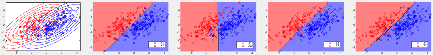
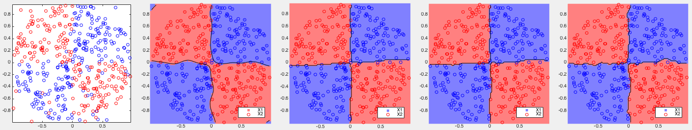
Example 1: Based on some 2-D training datasets, four different binary classifiers are tested. The correct rates of each of the four methods are listed below, together with the corresponding partitionings of the 2-D space shown in the figures.
 |
(191) |
![$\displaystyle {\bf m}_+=\left[\begin{array}{r}-1\\ 0\end{array}\right],\;\;\;\;...
...{\bf\Sigma}_-
=3\times \left[\begin{array}{cc}1&0.5\\ 0.5&0.5\end{array}\right]$](img713.svg) |
(192) |
 , slightly better than that
of the standard SVM
, slightly better than that
of the standard SVM  . But the kernel Bayes method I performs
poorly
. But the kernel Bayes method I performs
poorly  , as it is based only on the means of the two classes
without taking into consideration their covariances representing the
distribution of the data points.
, as it is based only on the means of the two classes
without taking into consideration their covariances representing the
distribution of the data points.
 , due to its quadratic term
in the decision function, the kernel Bayes I and II perform much
more poorly, but still slightly better than the SVM method.
, due to its quadratic term
in the decision function, the kernel Bayes I and II perform much
more poorly, but still slightly better than the SVM method.
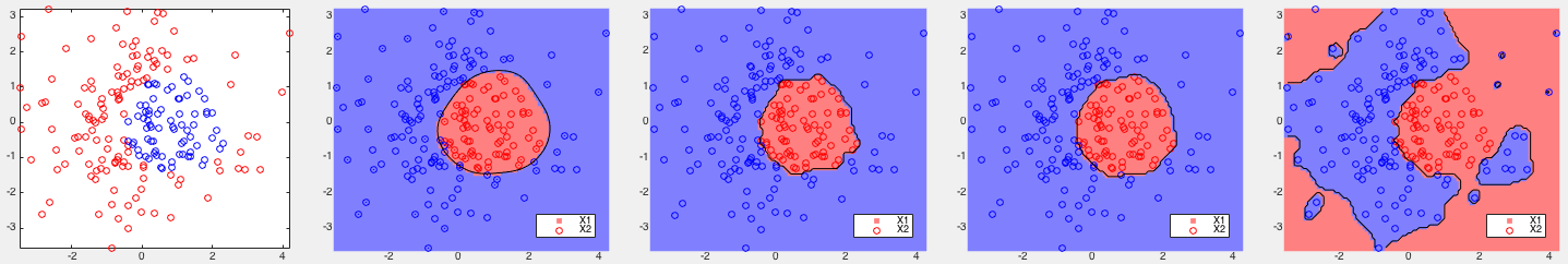
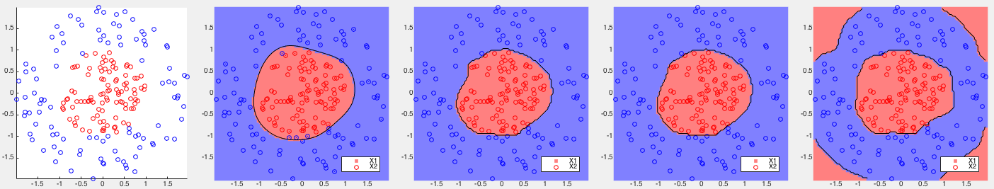
 , all three versions of the kernel Bayes
method (with
, all three versions of the kernel Bayes
method (with  ) achieve the perfect result with all points
of the two classes completely separate. However, the partitioning
of the space by the kernel Bayes III is highly fragmented, showing
a sign of overfitting.
) achieve the perfect result with all points
of the two classes completely separate. However, the partitioning
of the space by the kernel Bayes III is highly fragmented, showing
a sign of overfitting.
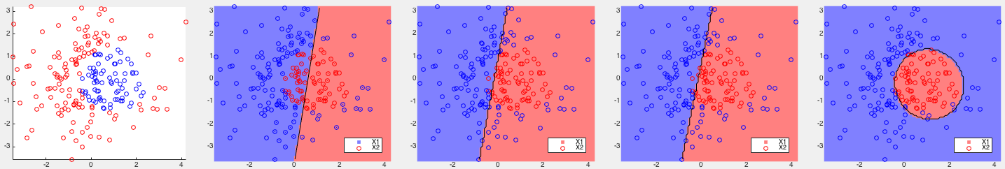
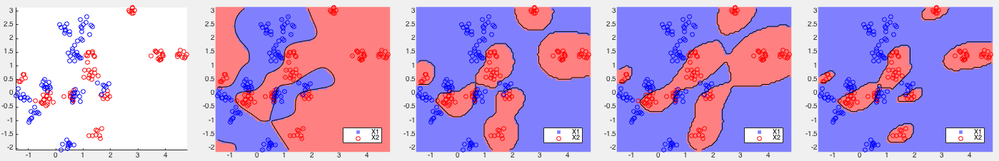
Example 2: The three datasets are generated using the Matlab
code on
this site.
A parameter value is used for the three versions of the
kernel Bayes method.
 |
(193) |
As the data are not linearly separable, all methods performed poorly except kernelized Bayes Type III with a second order term in the decison function.
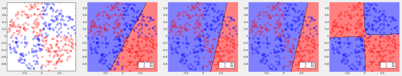
All four methods performed very well, but all three variations of the kernelized Bayes method achieved higher correct rates than the SVM.
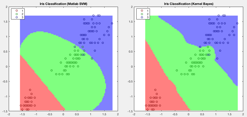
Example 3: The classification results of Fisher's iris data by
the SVM method (Matlab function fitcsvm) and the kernel Bayes
methods are shown below. This is an example used to illustrate the
SVM method in the
documentation of fitcsvm.
In this example only two (3rd and 4th) of the four features are used, with half of the samples used for training while the other half for testing. Note that the second class (setosa in green) and third class (versicolor in blue) not linearly separable can be better separated by the kernel Bayes method.


![$\displaystyle {\bf w}^T{\bf x}+w
=\left[{\bf\Sigma}^{-1}({\bf m}_+-{\bf m}_-)\right]^T{\bf x}+w$](img683.svg)
![$\displaystyle \left[{\bf UU}^T\left(\frac{1}{N_+}\sum_{{\bf x}_+}{\bf x}_+
-\frac{1}{N_-}\sum_{{\bf x}_-}{\bf x}_-\right)\right]^T{\bf x}+w$](img684.svg)


