Next: Kernelized Bayes classifier Up: Support Vector machine Previous: Sequential Minimal Optimization (SMO)
CrammerSinger WestonWatkins WangXue Bredensteiner
The SVM method is inherently a binary classifier, but it can be
adapted to classification problems of more than two classes. In
the following, we consider a general K-class classifier based on a
training set
![${\bf X}=[{\bf x}_1,\cdots,{\bf x}_N]$](img9.svg) , of which each
sample
, of which each
sample  is labeled by
 to indicate
 .
.
We first consider two straight forward and imperical methods for multiclass classification based directly on binary SVM.
Any unlabeled  is classified to a class which receives
the maximum votes out of the
is classified to a class which receives
the maximum votes out of the  binary classifications
between every pair of the
binary classifications
between every pair of the  classes.
This method converts a K-class problem ( ) into K binary
problems. First, we regroup the classes
) into K binary
problems. First, we regroup the classes
 into
two classes
into
two classes  and
and
 and
find the corresponding decision function
and
find the corresponding decision function
 representing
quantitatively to what extent a given belongs to class
(if
representing
quantitatively to what extent a given belongs to class
(if
 ), instead of
  containing all
remaining
containing all
remaining  classes (if
 ). After this process
has been carried out for all
). After this process
has been carried out for all
 , the can be
classified as below:
, the can be
classified as below:
if then then |
(159) |
We further consider another method for multiclass classifiction
by directly generalizing the binary SVM so that the decision
margin between any two of the classes is maximized. First,
we define a linear function for each of the classes:
 |
(160) |
 and
and  are determined during the
training set, any unlabeled point can be classified as
below:
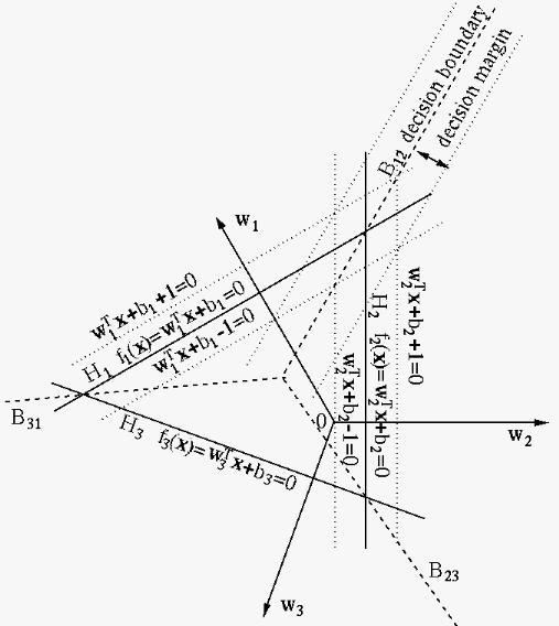
The figure below illustrates the classification of
are determined during the
training set, any unlabeled point can be classified as
below:
The figure below illustrates the classification of  classes
in
classes
in  dimensional feature space. Here each straight lines
  (plane or hyperplane if
  ) is determined by equation
 , with
normal direction in and distance
, with
normal direction in and distance
 to the origin (same as in
Eq. (65)).
to the origin (same as in
Eq. (65)).
According to the classification rule in Eq. (161),
the 2-D feature space is partitioned into three regions each for
one of the classes by the decision boundaries
 , of which boundary
  between classes
 and
and  is composed of all points
 satisfying
 . Same as in binary SVM,
we further define for each of the classes two additional
straight lines (planes or hyperplanes if ) parallel to
, denoted by
. Same as in binary SVM,
we further define for each of the classes two additional
straight lines (planes or hyperplanes if ) parallel to
, denoted by  and represented by equations
 . Their distances
to can be found as (same as in Eq. (70)):
. Their distances
to can be found as (same as in Eq. (70)):
 |
(162) |
 and
and  futher determine two straight
lines parallel to the decision boundary
futher determine two straight
lines parallel to the decision boundary  , defining the
decision margin between the support vectors of and .
It can be seen that this decision margin is monotonically related
to both
, defining the
decision margin between the support vectors of and .
It can be seen that this decision margin is monotonically related
to both
 and
and
 , which can
be maximized by minimizing both
, which can
be maximized by minimizing both
 and
and
 .
.
Now the multiclass classification problem can be formulated as
to find the parameters and for all
so that
 is minimized
and thereby the decision margins for all boundaries
between and are maximized, under the constraint that
every training sample labeled by
is minimized
and thereby the decision margins for all boundaries
between and are maximized, under the constraint that
every training sample labeled by  is correctly
classified with a decision margin of 1 (the distance between the
support vectors on both sides of is 2):
is correctly
classified with a decision margin of 1 (the distance between the
support vectors on both sides of is 2):
minimize: |
 |
||
| subject to: |
 |
(163) |
Similar to Eq. (115) in soft margin SVM, the
contraints of the optimization problem above can be relaxed by
including in each contraint an extra error term
 ,
which is to be minimized. Now the problem can be reformulated as
,
which is to be minimized. Now the problem can be reformulated as
| minimize: |
 |
||
| subject to: |
 |
||
 |
|||
 |
(164) |
The Lagrangian function of this constrained optimization problem is
 |
 |
 |
|
 |
![$\displaystyle \sum_k\sum_n \alpha_{nk}\left[ ({\bf w}_{y_n}-{\bf w}_k)^T{\bf x}_n
+b_{y_n}-b_k-2+\xi_{nk}\right]-\sum_k\sum_n \beta_{nk}\xi_{nk}$](img635.svg) |
(165) |
 |
|||
 |
|||
|
(166) |
 |
(167) |
 |
(168) |
 |
(169) |
 |
(170) |
![$\displaystyle {\bf W}=[{\bf w}_1,\cdots,{\bf w}_K]$](img642.svg) |
(171) |
is classified to class if
 .
.
The training of the classifier is to find all weight vectors in
 based on the training dataset. To do so, we first define
a cost function
based on the training dataset. To do so, we first define
a cost function
////
 then
then