K Nearest Neighbor and Minimum Distance Classifiers

Here we first consider a set of simple supervised classification algorithms that assign an unlabeled sample ${\bf x}$ to one of the $K$ known classes based on set $N$ of training samples ${\bf X}=[{\bf x}_1,\cdots,{\bf x}_N]$, where each sample ${\bf x}_n$ is labeled by $y_n=k\in\{1,\cdots,K\}$, indicating it belongs to class $C_k$.

• k Nearest neighbors (k-NN) Classifier

  Given an unlabeled pattern ${\bf x}$, we first find its $k$ nearest neighbors in the training dataset, and then assign ${\bf x}$ to one of the $K$ classes by a majority vote of the $k$ neighbors based on their class labelings. The voting can be weighted so that closer neighbors are more heavily weighted than those that are farther away. In particular, when $k=1$, ${\bf x}$ is assigned to the class of its closest neighbor.

  While the k-NN method is simple and straight forward, its computational cost is high as classifying any unlabeled pattern ${\bf x}$ requires computing distances to all data points in the training set.

• Minimum Distance Classifier

  Given a set of training data points $\{{\bf x}_1,\cdots,{\bf x}_{N_k}\}$ all belonging to the kth class $C_k$ ( $k=1,\cdots,K$), we can find their mean and covariance to represent the class:

  $${\bf m}_k=\frac{1}{N_k}\sum_{n=1}^{N_k} {\bf x}_n,\;\;\;\;\;\;\; ... ...igma}_k=\frac{1}{N_k}\sum_{n=1}^{N_k} ({\bf x}_n-{\bf m})^T ({\bf x}_n-{\bf m})$$ (1)

  Any unlabeled data point ${\bf x}$ can be classified to one of the $K$ classes based on certain distance $d({\bf x},\,C_k)$ between ${\bf x}$ and each of class $C_k$:

  $$\;\;d({\bf x},C_k)=min \{d({\bf x},C_i)\;\;i=1,\cdots,C \} \;\;\;\; \;\;{\bf x}\in C_k$$ (2)

  We could simply use the Euclidean distance $d_E({\bf x},{\bf m}_k)$ between ${\bf x}$ and ${\bf m}_k$. But such a classification may not reliable as Euclidean distance does not take into consideration the covariance ${\bf\Sigma}_k$ representing how the $N_k$ samples are distributed in the feature space, as illustrated by the following example.

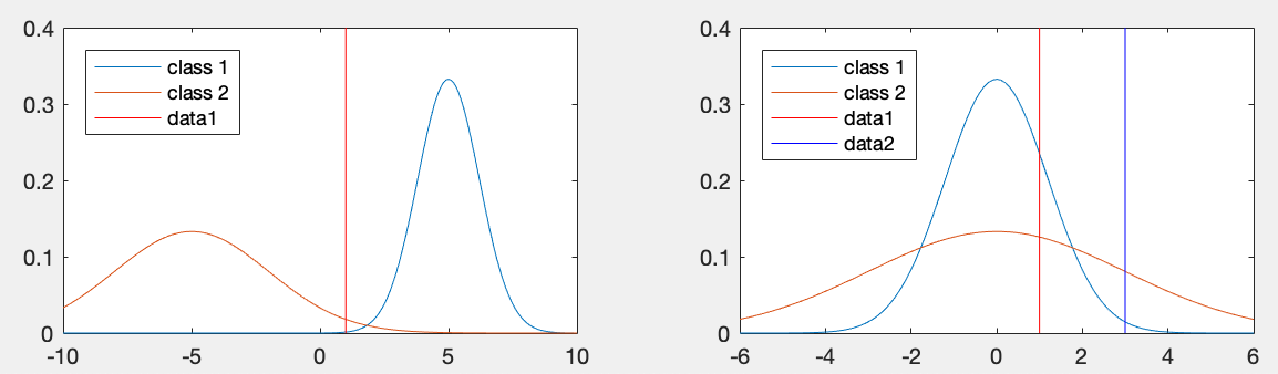
  Example 1: As illustrated in the figure below (left plot), a point $x=1$ in 1-D space is to be classified into one of the two classes represented by their corresponding Gaussian pdfs:

  $$C_1\sim{\cal N}( 5, 1.2^2),\;\;\;\;\;\;\;\;\;\;\;\;\; C_2\sim{\cal N}(-5, 3^2)$$ (3)

  If only the two means $m_1=5$ and $m_2=-5$ are considered, we have $d_E(x,\,m_1)=4\;<\;d_E(x,\,m_2)=6$, i.e., $x=1$ is closer to $m_1$ than $m_2$ and therefore should be classified to class $C_1$. However, as shown in the plot, $x$ should be classified to class $C_2$, if the variances $\sigma_1=1.2$ and $\sigma_2=3$ are also taken into consideration.

  

  We see the distance $d({\bf x},\,C_k)$ should be positively related to $d_E(x,\,m_k)$, but inversely related to $\sigma_k$, i.e., we can define $d(x,C_k)=(x-m_k)^2/\sigma_k^2$. Based on this distance, we find $d(x_1,\,m_1)=11.11 \;>\;d(x_1,\,m_2)=4.0$, i.e., $x=1$ should be classified to $C_2$.

  In a higher dimensional feature space, we can carry out classification based on the more generally defined Mahalanobis distance between a point ${\bf x}$ and a distribution represented by ${\bf m}_k$ and ${\bf\Sigma}_k$:

  $$d_M({\bf x},C_k)=({\bf x}-{\bf m}_k)^T{\bf\Sigma}_k^{-1}({\bf x}-{\bf m}_k)$$ (4)

  Example 2: As illustrated in the above figure (right plot), two samples $x_1=1$ and $x_2=3$ are to be classified into either of two classes:

  $$C_1\sim{\cal N}(0, 1.2^2),\;\;\;\;\;\;\;\;\;\;\;\;\; C_2\sim{\cal N}(0, 3^2)$$ (5)

  As the two means $m_1=m_2=0$ are the same, $\vert x_i-m_1\vert^2=\vert x_i-m_2\vert^2$ for both samples $x_1$ and $x_2$, they are both classified into $C_2$ with a greater variance $\sigma_2\;> \;\sigma_2$ therefore smaller Mahalanobis distances:

  $$\left\{ \begin{array}{l} d_M(x_1,\,C_1)=\frac{(x_1-m_1)^2}{\s... ...{(x_1-m_1)^2}{\sigma_2^2}=\frac{3^2}{9}=1.00 \end{array}\right.$$ (6)

  However, as shown in the plot, $x_1=1$ should be classified to $C_1$. We therefore see that sometimes the Mahalanobis distance is not reliable for classification, and some better method need to be considered, as discussed later.