Hierarchical (Tree) Classifiers

Both supervised classification and unsupervised clustering can be carried out in a hierarchical fashion to classify the input patterns or group them into clusters, very much like the hierarchy of biological classifications with different taxonomic ranks (domain, kingdom, phylum, class, order, family, genus, and species).

• Unsupervised clustering

  The hierarchical clustering can be obtained in either a top-down or bottom up manner.

  • Top-down method:

    All patterns in the data set are initially treated as a single cluster as the root of the tree, which is then subdivided (split) into a set of two or more smaller clusters, each represented as a node in the tree structure. This process is carried out recursively until eventually each cluster contains only one pattern, represented as a leaf node of the tree.

  • Bottom-up method:

    every pattern in the data set is initially treated as a cluster as a leaf node of the tree, which will then be merged to form larger clusters. Again, this process is carried out recursively until eventually all patterns are merged into a single cluster at the root of the tree.

  In either the top-down or the bottom-up method, the specific method for the splitting or merging at each tree node is based on certain similarity measurement such as the distance between two clusters. The resulting tree structure obtained by either method can then be truncated at any level between the root and the leaf nodes to obtain a set of clusters, depending on the desired number and sizes of these clusters.

• Supervised classification

  If labeled training data are available, both the top-down and the bottom-up clustering methods can also be used in the training stage of the supervised classification methods, with the only difference that now the splitting or merging is applied to labeled classes instead of individual patterns, and each leaf node represents one of the classes, rather than a single pattern. After the tree structure is obtained, the training is complete and any unlabeled pattern can be classified at the tree root and then subsequently the tree nodes at lower levels until it is classified into one of the leaf nodes of the tree, corresponding to a specific class.

  This hierarchical classification method is especially useful when the number of classes and the number $D$ of feature are both large. In this case it may be very difficult to select a subset of $d<D$ features good for separating all classes for a single-level classifier, by which all classes need to be classified at the same time, requiring, most likely, all $N$ features. However, for a tree classifier, since each node is a two-class classifier, it is possible to select a small number of $d\ll D$ features that are most relevant and suitable to represent the two subsets of classes.

In the following we consider both the bottom-up and top-down methods for hierarchical clustering/classification.

Bottom-Up method

The bottom-up hierarchical classifier is trained based on $K$ classes $C_1,\cdots,C_K$, each containing $n_k$ ( $k=1,\cdots,K$) labeled patterns ${\bf x}\in C_k$.

1. Compute the $K(K-1)/2$ pairwise Bhattacharyya distances between every two classes $C_i$ and $C_j$:

   $$d_B(C_i,C_j) =\frac{1}{4}({\bf m}_i-{\bf m}_j)^T\left[\frac{{\bf\... ...vert{\bf\Sigma}_i\right\vert\;\left\vert{\bf\Sigma}_j\right\vert)^{1/2}}\right]$$ (194)

2. Merge the two classes corresponding to the smallest $d_B$ to form a new class $C_i \cup C_j = C_k$, compute its mean and covariance:

   $${\bf m}_k=\frac{1}{n_i+n_j}[n_i {\bf m}_i+n_j {\bf m}_j]$$ (195)

   and

   $${\bf\Sigma}_k=\frac{1}{n_i+n_j} [n_i (\Sigma_i+({\bf m}_i-{\bf m}... ...i-{\bf m}_k)^T)+ n_j (\Sigma_j+({\bf m}_j-{\bf m}_k)({\bf m}_j-{\bf m}_k)^T ) ]$$ (196)

   Delete the old classes $C_i$ and $C_j$. Now there are $K-1$ classes left.

3. Compute the distance between the new class $C_k$ and all $K-2$ remaining classes.

4. Repeat the previous steps until eventually all classes are merged into a single group containing all $K$ classes, the binary tree structure is thus obtained.

Top-Down method

Generate a binary tree by recursively partitioning all classes into two sub-groups with the maximum Bhattacharyya distance

1. Compute the between-class scatter matrix ${\bf S}_B$ of the $K$ classes, find its maximum eigenvalue $\lambda_i$ and the corresponding eigenvectors ${\bf v}_i$;

2. Project all data points onto ${\bf v}_1$:

   $$y_n={\bf x}^T_n {\bf v}\;\;\;\;\;\;(n=1,\cdots,N)$$ (197)

3. Sort all data points $\{ y_1,\cdots,y_N\}$ along this 1-D space and partition them into two subgroups with maximum Bhattacharyya (between-group) distance.

4. Carry out the steps above recursively to each of the two subgroups, until eventually every subgroup contains only one classes

Once the hierarchical structure is constructed by either the bottom-up or top-down method, we need to build a binary classifier at each node of structure, by which any given pattern is classified into either the left group $G_l$ or right group $G_r$:

• According to the specific classification method used, find the discriminant functions $D_l({\bf x})$ and $D_r({\bf x})$ for the two subgroups based on the training data.

• Select the best $d<D$ features most suitable for separating the two groups $G_l$ and $G_r$, based on any of the feature selection methods such as those listed below:
  • Choosing $d$ features directly from the $D$ original ones using between-class distance (Bhattacharrya distance) as the criterion,

  • Carry out KLT based on the between-class scatter matrix ${\bf S}_B$ and use the first $d$ principal components for the binary classification.
  As here only two groups of classes need to be distinguished, the number of features $M$ can be expected to be small.

• Any unlabeled pattern ${\bf x}$ enters the classifier at the root of the tree and is classified to either the left or the right sub-group of the node according to the discriminant function

  $${\bf x} \in \left\{ \begin{array}{ll} G_l & if \;\;D_l({\bf x}) > D_r({\bf x}) \\ G_r & if \;\;D_r({\bf x}) < D_l({\bf x}) \end{array} \right.$$ (198)

  This process is carried out recursively at each of the subsequent nodes until eventually ${\bf x}$ reaches one of the leaf nodes corresponding to a single class, to which the sample ${\bf x}$ is therefore classified.

Example

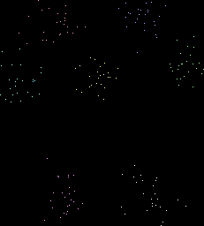
The hierarchical clustering method is applied to a dataset composed of seven normally distributed clusters each containing 25 sample vectors in an $N=4$ dimensional space. The PCA method is used to project the data in 4-D space into a 2-D space spanned by the first two principal components, as shown below:

The clustering result is shown below. Each column in the display represents the four components of a 4-D vector, color coded by a spectrum from red (low values) through green (middle) to blue (high values).

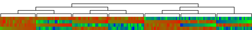
See more examples in clustering analysis applied to gene data analysis in bioinformatics.

An example of this method is available here.