Gaussian Process Classifier - Multi-Class

The binary GPC considered previously can be generalized to multi-class GPC based on softmax function, similar to the how binary classification based on logistic function is generalized to multi-class classification. First of all, we define the following variables for each class $C_k,\; (k=1,\cdots,K)$ of the $K$ classes $\{C_1,\cdots,C_K\}$:

• Class labeling:

  Binary labeling ${\bf y}_k=[y_{1k},\cdots,y_{Nk}]^T$ indicating whether each of the $N$ samples in the training set ${\bf X}=[{\bf x}_1,\cdots,{\bf x}_N]$ belongs to $C_k$:

  $$y_{nk}=\left\{\begin{array}{ll} 1&\mbox{if ${\bf x}_n\in C_k$}\\ 0&\mbox{if ${\bf x}_n\notin C_k$}\end{array}\right.$$ (297)

  In other words, each training sample ${\bf x}_n\in C_k$ is labeled by $K$ binary variables $y_{nk}=1$ and $y_{nl}=0$ for all $l=1,\cdots,K,\;l\ne k$ (same as in softmax regression), as well as an integer labeling $y_n=k$.

• Latent functions:

  Latent function ${\bf f}_k=[f_{1k},\cdots,f_{Nk}]^T$, of which the nth component $f_{nk}=f_k({\bf x}_n)\;(n=1,\cdots,N)$ is kth Gaussian process associated with $C_k$ evaluated at the nth training sample ${\bf x}_n$ in the training set ${\bf X}=[{\bf x}_1,\cdots,{\bf x}_N]$.

• Probability modeling:

  Probability ${\bf p}_k=[p_{1k},\cdots,p_{Nk}]^T$, of which the nth component $p_{nk}\;(n=1,\cdots,N)$ is the probability for ${\bf x}_n\in C_k$, modeled by the solftmax function based on $f_{nk}$ (same as in Eq. (237) in softmax regression):

  $$p_{nk}=p(\hat{y}=k\vert{\bf x}_n) =\frac{e^{f_{nk}}}{\sum_{l=1}^K e^{f_{nl}}}, \;\;\;\;\;\;(k=1,\cdots,K,\;\;n=1,\cdots,N)$$ (298)

  Note that if $y_{nk}=1$ then necessarily $y_{nl}=0$ for all $l=1,\cdots,K$ but $l\ne k$, i.e., the $K$ variables $y_{n1},\cdots,y_{nK}$ are not independent. given $p(y_{nk}=1)$, we do not need to consider $p(y_{nl}=0)$ for any $l\ne k$.

The probability for ${\bf x}_n$ to be correctly classified into class $C_{y_n}$ can be written as the following product of $K$ factors (of which $K-1$ are equal to 1, same as Eq. (238) in softmax regression):

$$p(\hat{y}=y_n\vert{\bf x}_n,{\bf f}) =\prod_{k=1}^K p(y_{nk}=1\vert{\bf x}_n,{\bf f})^{y_{nk}} =\prod_{k=1}^K p_{nk}^{y_{nk}}$$ (299)

Based on ${\bf y}_k$, ${\bf f}_k$, and ${\bf p}_k$ for all $k=1,\cdots,K$, we further define the following $KN$ dimensional vectors:

$${\bf y}=\left[\begin{array}{c}{\bf y}_1\\ \vdots\\ {\bf y}_K\end{... ...p_{11}\\ \vdots\\ p_{N1}\\ \vdots\\ p_{1K}\\ \vdots\\ p_{NK} \end{array}\right]$$ (300)

The posterior of ${\bf f}$ given the training set ${\cal D}$ can be found based on the Bayesian theorem as (same as in Eq. (267) in the binary case):

$$p({\bf f}\vert{\cal D})=p({\bf f}\vert{\bf X},{\bf y}) =\frac{p({... ...{p({\bf y}\vert{\bf X})} \propto p({\bf y}\vert{\bf f})\;p({\bf f}\vert{\bf X})$$ (301)

We first find the likelihood based on all $p_{nk}$ (same as Eq. (239) in softmax regression):

$$L({\bf f}\vert{\bf y})\propto p({\bf y}\vert{\bf f}) =\prod_{n=1}... ...\prod_{k=1}^K \left( \frac{e^{f_{nk}}}{\sum_{h=1}^K e^{f_{nh}}}\right)^{y_{nk}}$$ (302)

As each sample ${\bf x}_n$ belongs to only one of the $K$ classes, only one of $\{y_{n1},\cdots,y_{nK}\}$ can be 1 while all others are 0, consequently, the product above contains only $N$ probabilities raised to the power of $y_{nk}=1$, each for one of the $N$ samples belonging to a certain class, while all other probabilities raised to the power of $y_{nk}=0$ become 1 and not considered.

We next assume the prior probability of the latent function ${\bf f}_k$ for each class $C_k$ to be a zero-mean Gaussian process $p({\bf f}_k\vert{\bf X})={\cal N}({\bf0},{\bf\Sigma}_k)$, where the covariance matrix ${\bf\Sigma}_k$ is constructed based on the squared exponential (SE) for its mn-th component:

$$cov(f_k({\bf x}_m),f_k({\bf x}_n))=cov(f_{mk},f_{nk}) =k({\bf x}_... ...}\vert\vert{\bf x}_m-{\bf x}_n\vert\vert^2\right), \;\;\;\;\;\;(m,n=1,\cdots,N)$$ (303)

Then the prior of ${\bf f}$ containing all $K$ such latent functions is also a Gaussian $p({\bf f}\vert{\bf X})={\cal N}({\bf0},{\bf K})$, where ${\bf0}$ is a KN-dimensional zero vector and ${\bf K}$ is a $KN \times KN$ block diagonal matrix

$${\bf K}=\left[\begin{array}{cccc}{\bf K}_1 & {\bf0} &\cdots &{\bf... ...ots & \ddots & \vdots \\ {\bf0} & \cdots & {\bf0} &{\bf K}_K\end{array}\right]$$ (304)

with ${\bf K}_1=\cdots={\bf K}_K$ as defined in Eq. (254) on the diagonal. All off-diagonal blocks are zero as the latent functions of different classes are uncorrelated.

Having found both the likelihood $p({\bf y}\vert{\bf f})$ and prioor $p({\bf f}\vert{\bf X})$, we can write the posterior as

$$p({\bf f}\vert{\cal D}) \propto p({\bf f}\vert{\bf X},{\bf y})\pr... ...^{f_{nk}}}{\sum_{h=1}^K e^{f_{nh}}} \right)^{y_{nk}} {\cal N}({\bf0},\,{\bf K})$$ (305)

We note that the likelihood $p({\bf y}\vert{\bf f})$ is not Gaussian, as $y_{nk} \in\{0,\,1\}$ is a binary labeling, instead of a continuous variable. As a product of the Gaussian prior and non-Gaussian likelihood, the posterior $p({\bf f}\vert{\cal D})$ is not a Gaussian process either. However, for convnience, we still assume it is approximately Gaussian $p({\bf f}\vert{\cal D})\approx {\cal N}({\bf f},\,{\bf m}_{f\vert D},\,{\bf\Sigma}_{f\vert D})$, of which the mean ${\bf m}_{f\vert D}$ and covariance ${\bf\Sigma}_{f\vert D}$ are to be found.

Taking log of the posterior, we get

$$\psi({\bf f}) = \log p({\bf f}\vert{\cal D}) =\log p({\bf y}\vert{\bf f}) + \log ... ...}\left(f_{nk}-\log\sum_{h=1}^K e^{f_{nh}}\right) +\log {\cal N}({\bf0},{\bf K})$$

$$= {\bf y}^T{\bf f}-\sum_{n=1}^N \log \sum_{h=1}^K e^{f_{nh}} -\frac... ...\pi)-\frac{1}{2}\log\vert{\bf K}\vert -\frac{1}{2}{\bf f}^T {\bf K}^{-1}{\bf f}$$ (306)

where we have used the fact that $\sum_{k=1}^K y_{nk}=1$. The gradient of $\psi({\bf f})$ is

$${\bf g}_\psi = \frac{d}{d{\bf f}} \psi({\bf f})=\frac{d}{d{\bf f}} \left( {\bf y... ...rac{1}{2}\log\vert{\bf K}\vert -\frac{1}{2}{\bf f}^T {\bf K}^{-1}{\bf f}\right)$$

$$= {\bf y}-{\bf p}-{\bf K}^{-1}{\bf f}$$ (307)

where the second term ${\bf p}$ comes from

$$\sum_{n=1}^N \frac{d}{d{\bf f}} \log \sum_{h=1}^K e^{f_{nh}} =\su... ...in{array}{c}0\\ \vdots\\ 0\\ p_{nk}\\ 0\\ \vdots\\ 0\end{array}\right]={\bf p}$$ (308)

Note that ${\bf p}={\bf p}({\bf f})$ is a function of ${\bf f}$.

As the posterior $p({\bf f}\vert{\cal D})\approx{\cal N}({\bf m}_{f\vert D},{\bf\Sigma}_{f\vert D})$ is approximated as a Gaussian, which reaches maximum at its mean ${\bf m}_{f\vert D}$, and so does the log prior $\psi({\bf f})=\log p({\bf f}\vert{\cal D})$, and the gradient of $\psi({\bf f})$ is zero at ${\bf f}={\bf m}_{f\vert D}$:

$${\bf g}_\psi({\bf f})\bigg\vert _{{\bf f}={\bf m}_{f\vert D}} ={\... ...bf m}_{f\vert D}} ={\bf y}-{\bf p}_{m_f}-{\bf K}^{-1}{\bf m}_{f\vert D}={\bf0},$$ (309)

i.e.,

$${\bf m}_{f\vert D}={\bf K}({\bf y}-{\bf p}_{m_f})$$ (310)

where ${\bf p}_{m_f}={\bf p}({\bf m}_{f\vert D})$ is the vector defined above evaluated at ${\bf f}={\bf m}_{f\vert D}$.

We further get the Hessian matrix of $\psi({\bf f})$:

$${\bf H}_\psi({\bf f})=\frac{d^2}{d{\bf f}^2} \psi({\bf f}) =\frac... ...-1}{\bf f}-{\bf p} \right) =-{\bf K}^{-1} -{\bf W}=-{\bf\Sigma}_{f\vert D}^{-1}$$ (311)

The last equality is due to the property of the Gaussian distribution (see Appendix), from which we get the KN by KN covariance matrix of $p({\bf f}\vert{\cal D})$:

$${\bf\Sigma}_{f\vert D}=-{\bf H}^{-1}_\psi({\bf f})=({\bf K}^{-1}+{\bf W})^{-1}$$ (312)

Here ${\bf W}=d{\bf p}/d{\bf f}$ is a $KN \times KN$ Jacobian matrix of ${\bf p}$, of which the $ijkl$-th component $(i,j=1,\cdots,N,\;\;k,l=1,\cdots,K)$ is:

$$\frac{\partial}{\partial f_{jl}} p_{ik} = \frac{\partial}{\partial f_j^l}\left[\frac{e^{f_{ik}}}{\sum_{h=1}... ..._{kl}-e^{f_{ik}}e^{f_{jl}}} {\left(\sum_{h=1}^K e^{f_{ih}}\right)^2}\delta_{ij}$$

$$= \left[\frac{e^{f_{ik}}}{\sum_{h=1}^K e^{f_{ih}}}\delta_{kl} -\fra... ...h}}\right)^2}\right] \delta_{ij} =(p_{ik}\delta_{kl}-p_{ik} p_{jl})\delta_{ij},$$ (313)

and ${\bf W}$ can be written also in two terms:

$${\bf W}=diag({\bf p})-{\bf PP}^T$$ (314)

where the first term $diag({\bf p})$ is a diagnal matrix containing all $KN$ components of ${\bf p}$ along the diagnal ($k=l$ and $i=j$), and ${\bf P}$ in the second term is a KN by N matrix composed of $K$ $N\times N$ diagonal matrices $diag({\bf p}_k)$:

$${\bf P}=\left[\begin{array}{c}diag({\bf p}_1)\\ \vdots\\ diag({\... ...& \vdots\\ 0 & \cdots & 0 & p_{Nk} \end{array}\right],\;\;\;\;\;(k=1,\cdots,K)$$ (315)

so that

$${\bf PP}^T=\left[\begin{array}{c}diag({\bf p}_1)\\ \vdots\\ diag... ...diag({\bf p}_K) diag({\bf p}_1) & \cdots & diag({\bf p}_K^2) \end{array}\right]$$ (316)

with

$$diag({\bf p}_k) diag({\bf p}_l)=\left[\begin{array}{cccc} p_1^kp_... ...& \vdots & \ddots & \vdots \\ 0 & \cdots & 0 & p_{Nk}p_{Nl} \end{array}\right]$$ (317)

Having found both the gradient ${\bf g}_\psi={\bf y}-{\bf p}-{\bf K}^{-1}{\bf f}$ and Hessian ${\bf H}_\psi=-({\bf K}^{-1}+{\bf W})$, we can further find the mean ${\bf m}_{f\vert D}$ at which $\psi({\bf f})$ achieves maximum by the following iteration of Newton's method:

$${\bf f}_{n+1} = {\bf f}_n-{\bf H}_\psi^{-1}{\bf g}_\psi ={\bf f}_n+({\bf K}^{-1}+{\bf W})^{-1}({\bf y}-{\bf K}^{-1}{\bf f}_n-{\bf p})$$

$$= {\bf f}_n+({\bf K}^{-1}+{\bf W})^{-1}(-({\bf K}^{-1}+{\bf W}){\bf f}_n+{\bf W}{\bf f}_n+{\bf y}-{\bf p})$$

$$= ({\bf K}^{-1}+{\bf W})^{-1}({\bf W}{\bf f}_n+{\bf y}-{\bf p})$$ (318)

We note that during the iteration, we need to update not only ${\bf f}$, but also ${\bf p}$ as a functions of ${\bf f}$ given in Eq. (308).

Now that we have got both ${\bf m}_{f\vert D}$ and ${\bf\Sigma}_{f\vert D}$ of ${\bf f}$, we can further get ${\bf m}_{f_*}$ and ${\bf\Sigma}_{f_*}$ of ${\bf f}_*$:

• Get mean ${\bf m}_{f_*}$:

  Similar to Eq. (292) in the binary case, we have the following based on ${\bf f}={\bf K}({\bf y}-{\bf p})$ in Eq. (310):
  

  $${\bf m}_{f_*} = E_f({\bf m}_{f_*\vert f}) =E_f ({\bf K}_*^T{\bf K}^{-1}{\bf f})={\bf K}_*^T{\bf K}^{-1}E_f({\bf f})$$

  $$= {\bf K}_*^T{\bf K}^{-1}\,[{\bf K}({\bf y}-{\bf p}_{m_f})] ={\bf K}_*^T({\bf y}-{\bf p}_{m_f})$$ (319)

  
  As the $K$ classes are uncorrelated, i.e., ${\bf K}$ is block-diagonal, the above can be separated into $K$ equations each for one of the classes:

  $${\bf m}_{f_*^k}=({\bf K}_*^k)^T({\bf y}^k-{\bf p}^k), \;\;\;\;\;\;(k=1,\cdots,K)$$ (320)

• Get covariance ${\bf\Sigma}_{f_*}$:

  Similar to Eq. (294) in the binary case, we have the following based on ${\bf\Sigma}_{f\vert D}=({\bf K}^{-1}+{\bf W})^{-1}$ in Eq. (312):

  $${\bf\Sigma}_{m_{f_*\vert f}} ={\bf K}_*^T {\bf K}^{-1}\,{\bf\Sigm... ...}_* ={\bf K}_*^T {\bf K}^{-1} ({\bf K}^{-1}+{\bf W})^{-1} {\bf K}^{-1}{\bf K}_*$$ (321)

  where ${\bf W}=diag({\bf p})-{\bf PP}^T$ is given in Eq. (314) with ${\bf p}$ evaluated at ${\bf m}_{f\vert D}$. Then, similar to Eq. (294), we get

  $${\bf\Sigma}_{f_*}={\bf K}_{**}-{\bf K}_*^T({\bf K}+{\bf W}^{-1})^{-1}{\bf K}_*$$ (322)

Now we can further get the probability for ${\bf x}_*$ to belong to $C_k$ based on the softmax function in Eq. (298)

$$p_*^k=\frac{e^{m_{f_*}^k}}{\sum_{l=1}^K e^{m_{f_*}^l}}, \;\;\;\;\;\;(k=1,\cdots,K)$$ (323)

and classifiy ${\bf x}_*$ to class $C_k$ if $p_*^k=\max\{ p_*^1,\cdots,p_*^K \}$.

Moreover, the certainty or confidence of this classification result can be found from ${\bf\Sigma}_{f_*}$.

The Matlab code for the essential parts of the algorithm is listed below. First, the following code segment carries out the classification of $n$ given test samples based on the $N$ training set ${\cal D}=\{ {\bf X},{\bf y}\}$.

    K=Kernel(X,X);                        % covariance of prior of p(f|X)
    Ks=Kernel(X,Xs);
    Kss=Kernel(Xs,Xs);
    [meanf Sigmaf p W]=findPosteriorMeanMC(K,y,C);  
                                          % find mean and covariance of p(f|D), and W, p
    Sigmafy=Kss-Ks'*inv(K+inv(W))*Ks;     % covariance of p(f|D) 
    p=reshape(p,N,C);
    y=reshape(y,N,C);
    for k=1:C
        meanfD(:,k)=Ks'*(y(:,k)-p(:,k);   % mean of p(f_*|X_*,D) for kth class
    end
    for i=1:n                             % for each of n test samples
        d=sum(exp(meanfD(i,:)));          % denominator of softmax function
        [pmax k]=max(exp(meanfD(i,:))/d); % find class with max probability
        ys(i)=k;                          % label ith sample as member of kth class
        pr(i,k)=pmax;                     % probility of ith sample belonging to kth class 
    end

The code segment above calls the following function which computes the mean and covariance of $p({\bf f}\vert{\bf X},{\bf y})$ by Newton's method:

function [meanf Sigmaf p W]=findPosteriorMeanMC(K,y,C)     
    % find mean and covariance of p(f|X,y) by Newton's method, based on D={X,y}
    n=length(y);                    % number of training samples
    f0=zeros(n,1);                  % initial value of latent function
    f=zeros(n,1);        
    er=1;
    k=0;  
    while er > 10^(-9)              % find f that maximizes p(f|X,y)
        k=k+1;
        [p W]=findp(f,N,C);         % call function findp to find vector p and matrix W
        f=inv(inv(K)+W)*(W*f0+y-p); % iteratively update value of f
        er=norm(f-f0);              % difference between consecutive iterations
        f0=f;                       % update f
    end
    meanf=f;
    Sigmaf=inv(inv(K)+W);            
end

The following function called by the previous function finds vector ${\bf p}$ and matrix ${\bf W}=diag({\bf p})-{\bf PP}^T$:

function [p W]=findp(f,N,C)         % find vector p and matrix W=diag(p)-P*P'
    F=reshape(f,N,C)';              % kth row contains N samples of class k
    p=zeros(C,N);                   % initialize p
    for n=1:N                       % for each of N training samples
        d=sum(exp(F(:,n)));         % sum of all C terms in denominator
        for k=1:C                   % for all C classes 
            p(k,n)=exp(F(k,n))/d;
        end
    end
    P=[];
    for k=1:C                       % generate P
        P=[P; diag(p(k,:))];        % stack C diagonal matrices
    end
    p=reshape(p',N*C,1);            % convert p into a column vector
    W=diag(p)-P*P';                 % generate W matrix
end

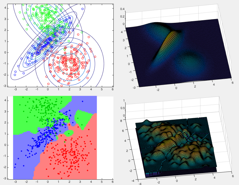
Example 1:

This example shows the classification result of the same dataset of three classes used before. The top two panels show the distributions of the three classes in the training data set. The bottom two panels show the classification results in terms of the partitioning of the feature space (bottom left) and the posterior distribution $p({\bf f}_*\vert{\bf X},{\bf y},{\bf X}_*)$ (bottom right), which can be compared with the distribution of the training set (top right). The confusion matrix of the classification result is shown below, with the error rate $30/600=0.045$:

$$\left[\begin{array}{rrr} 197 & 3 & 0 \\ 0 & 195 & 5 \\ 1 & 21 & 178 \\ \end{array}\right]$$ (324)

Example 2:

This example shows the classification of the XOR data set. The confusion matrix of the classification result is shown below, with the error rate $13/400=0.0325$:

$$\left[\begin{array}{rr} 193 & 7 \\ 6 & 194 \end{array}\right]$$ (325)

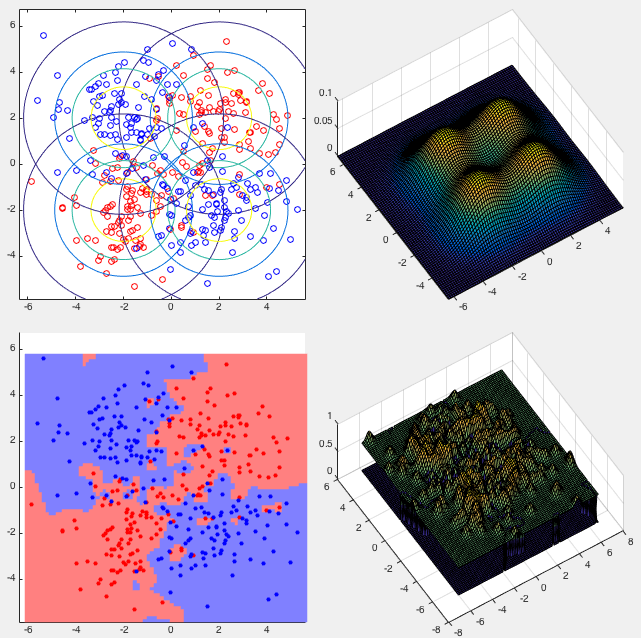
We see that in both examples, the error rates of the GPC method are lower than those of the naive Bayesian method. However, the naive Bayesian method does not have the overfitting problem, while in the method of GPC, we may need to carefully adjust the parameter of squared exponential for the kernel functions to make proper tradeoff between overfitting and error rate.