Gaussian Process Classifier - Binary

In both logistic regression and softmax regression considered previously, we convert the linear regression function $\hat{y}=f({\bf x})={\bf x}^T{\bf w}$ to the probability $p(\hat{y}=k\vert{\bf x},{\bf W})$ for ${\bf x}\in C_k$, by either the logistic function $\sigma(f({\bf x}))$ for binary classification, or the softmax function $s(f({\bf x}))$ for multiclass classification. Also, in Gaussian process regression (GPR), we treat the regression function $f({\bf x})$ as a Gaussian process. Now we consider the Gaussian process classification (GPC) based on the combination of both logistic/softmax regression and Gaussian process regression. We will consider binary GPC based on the logistic function in this section, and then multiclass GPC based on softmax function in the following section.

Here in binary GPC, we assume the training samples are labeled by 1 or -1 (instead of 0) for mathematical convenience, i.e., ${\bf x}_n\in C_+$ if $y_n=1$ or ${\bf x}_n\in C_-$ if $y_n=-1$. Similar to logistic programming, here we also convert the regression function $f({\bf x})$, now a Gaussian process, into the probability for ${\bf x}\in C_k$ by the logistic function $\sigma(f({\bf x}))$. However, as a function of this random argument, $\sigma(f({\bf x}))$ is also random. We therefore define $p(y=1\vert{\bf x},{\cal D})$ as the expectation of $\sigma(f({\bf x}))$ with respect to $f({\bf x})$:

$$p(y=1\vert{\bf x},{\cal D}) = E_f[\sigma(f({\bf x}))] =\int\sigma(f({\bf x}))\;p(f\vert{\bf x},{\cal D})\,d f$$ (265)

As function $f({\bf x})$ is marginalized (averaged out) in the integral above, it is hidden instead of explicitly specified, and is therefore called a latent function.

For the training set ${\bf X}=[{\bf x}_1,\cdots,{\bf x}_N]$, we define ${\bf f}({\bf X})=[f({\bf x}_1),\cdots,f({\bf x})]^T$, and express the probability above in vector form:

$$p({\bf y}=1\vert{\cal D})=E_f[ \sigma({\bf f}({\bf X})) ] =\int \sigma({\bf f}({\bf X}))\; p({\bf f}\vert{\cal D})\,d {\bf f}$$ (266)

where $p({\bf f}\vert{\cal D})$ is the posterior which can be found in terms of the likelihood $p({\bf y}\vert{\bf f})=L({\bf f}\vert{\bf y})$ and the prior $p({\bf f}\vert{\bf X})$ based on Bayes' theorem:

$$p({\bf f}\vert{\cal D})=p({\bf f}\vert{\bf X},{\bf y}) =\frac{p({... ...{p({\bf y}\vert{\bf X})} \propto p({\bf y}\vert{\bf f})\,p({\bf f}\vert{\bf X})$$ (267)

As always, the denominator ${p({\bf y}\vert{\bf X})}$ independent of ${\bf f}$ is dropped.

We first find the likelihood $p({\bf y}\vert{\bf f})$. The Gaussian process $f({\bf x})$ is mapped by the logistic function into the probability for $y=1$ for ${\bf x}\in C_+$, or $y=-1$ for ${\bf x}\in C_-$:

$$p(y=1\vert f({\bf x})) = \sigma(f({\bf x}))$$

$$p(y=-1\vert f({\bf x})) = 1-p(y=1\vert f({\bf x}) ) =1-\sigma(f({\bf x})) =\sigma(-f({\bf x}))$$ (268)

These two cases can be combined to get the conditional probability of $y$ given $f({\bf x})$:

$$p(y\vert f)=\sigma(y\,f({\bf x}) )=\sigma(y\,f) =\frac{1}{1+e^{-yf}}=\frac{e^{yf}}{1+e^{yf}}$$ (269)

The likelihood of ${\bf f}$ for all $N$ i.i.d. samples in the training set ${\bf X}$ is:

$$p({\bf y}\vert{\bf f})=\prod_{n=1}^N p(y_n\vert f_n) =\prod_{n=1}^N \sigma(y_n\,f_n)$$ (270)

We then consider the prior $p({\bf f}\vert{\bf X})$, which is assumed to be a zero-mean Gaussian $p({\bf f}\vert{\bf X})={\cal N}({\bf0},{\bf\Sigma}_f)$. Here the covariance matrix ${\bf\Sigma}_f$ can be constructed based on the training set ${\bf X}$, the same as in GPR. Specifically, the covariance between $f({\bf x}_m)$ and $f({\bf x}_n)$ in the mth row and nth column of ${\bf\Sigma}_f$ is modeled by the squared exponential (SE) kernel:

$$cov(f({\bf x}_m),f({\bf x}_n))=k({\bf x}_m,{\bf x}_n) =\exp\left(... ...}\vert\vert{\bf x}_m-{\bf x}_n\vert\vert^2\right), \;\;\;\;\;\;(m,n=1,\cdots,N)$$ (271)

Such a covariance matrix is desired for GPC as well as GPR, so that $f({\bf x}_m)$ and $f({\bf x}_n)$ are more correlated if ${\bf x}_m$ and ${\bf x}_n$ are close together, but less so if they are farther apart. However the justification for such a property is different. In GPR, this property is desired for the smoothness of the regression function; while here in GPC, this property is also desired so that function values $f({\bf x}_m)$ and $f({\bf x}_n)$ for two samples ${\bf x}_m$ and ${\bf x}_n$ close to each other in the feature space are more correlated and therefore the two samples are more likely to be classified into the same class, but less so if they are far apart.

Also, as discussed in GPR, here the parameter $a$ in the SE controls the smoothness of the function. If $a\rightarrow\infty$, the value of the SE approaches 1, then $f({\bf x}_m)$ and $f({\bf x}_n)$ are highly correlated and $f({\bf x})$ is very smooth; but if $a\rightarrow 0$, SE approaches 0, then $f({\bf x}_m)$ and $f({\bf x}_n)$ are not correlated and $f({\bf x})$ is no longer smooth. By adjusting $a$, a proper tradeoff can be made between overfitting and underfitting.

Having found both the likelihood $p({\bf y}\vert{\bf f})$ and the prior $p({\bf f})$, we can get the posterior in Eq. (267):

$$p({\bf f}\vert{\cal D}) \propto p({\bf y}\vert{\bf f})\,p({\bf f}\vert{\bf X}) =p({\bf y}\vert{\b... ...rt{\bf K}\vert^{1/2}} \exp\left(-\frac{1}{2}{\bf f}^T{\bf K}^{-1}{\bf f}\right)$$

$$\propto \prod_{n=1}^N\sigma(y_n\,f_n)\; \exp\left(-\frac{1}{2}{\bf f}^T{\bf K}^{-1}{\bf f}\right)$$ (272)

Note that the likelihood $p({\bf y}\vert{\bf f})$ is not Gaussian, as the binary labeling ${\bf y}$ of the training set ${\bf X}$ is not continuous. Consequently, the posterior $p({\bf f}\vert{\cal D})$, as a product of the Gaussian prior and non-Gaussian likelihood, is not Gaussian. However, we can carry out Laplace approximation and still approximate the posterior as a Gaussian:

$$p({\bf f}\vert{\cal D})\approx {\cal N}({\bf m}_{f\vert D},{\bf\Sigma}_{f\vert D})$$ (273)

of which the mean ${\bf m}_{f\vert D}$ and covariance ${\bf\Sigma}_{f\vert D}$ are to be obtained in the following. We further get the log posterior denoted by $\psi({\bf f})$:

$$\psi({\bf f})=\log\,p({\bf f}\vert{\cal D}) =\sum_{n=1}^N\log\sig... ...\pi)-\frac{1}{2}\log\vert{\bf K}\vert -\frac{1}{2}{\bf f}^T {\bf K}^{-1}{\bf f}$$ (274)

The two middle terms are constant independent of ${\bf f}$ and can therefore be dropped.

Now that the posterior $p({\bf f}\vert{\cal D})$ is approximated as a Gaussian, we can find the gradient vector ${\bf g}_\psi({\bf f})$ and Hessian matrix ${\bf H}_\psi({\bf f})$ of the log posterior (see Appendix):

$${\bf g}_{\psi}({\bf f}) = \frac{d}{d{\bf f}}\psi({\bf f}) =-{\bf\Sigma}^{-1}_{f\vert D} ({\bf f}-{\bf m}_{f\vert D})$$ (275)

$${\bf H}_{\psi}({\bf f}) = \frac{d^2}{d{\bf f}^2}\psi({\bf f}) =\frac{d}{d{\bf f}}{\bf g}_{\psi}({\bf f})=-{\bf\Sigma}_{f\vert D}^{-1}$$ (276)

On the other hand, we can also find ${\bf g}_{\psi}({\bf f})$ and ${\bf H}_{\psi}({\bf f})$ by directly taking the first and second order derivatives of the log posterior::

$${\bf g}_{\psi}({\bf f})=\frac{d}{d{\bf f}}\psi({\bf f}) =\frac{d}... ...ft(\frac{1}{2} {\bf f}^T{\bf K}^{-1}{\bf f}\right) ={\bf w}-{\bf K}^{-1}{\bf f}$$ (277)

$${\bf H}_{\psi}({\bf f})=\frac{d^2}{d{\bf f}^2}\psi({\bf f}) =\fra... ...ac{d}{d{\bf f}} \left( {\bf w}-{\bf K}^{-1}{\bf f}\right) ={\bf W}-{\bf K}^{-1}$$ (278)

where we have defined

$${\bf w}=\frac{d}{d{\bf f}}\log p({\bf y}\vert{\bf f}), \;\;\;\;\;... ...}=\frac{d^2}{d{\bf f}^2} \log p({\bf y}\vert{\bf f}) =\frac{d{\bf w}}{d{\bf f}}$$ (279)

are respectively the gradient vector and Hessian matrix of the log function

$$\log p({\bf y}\vert{\bf f})=\log \prod_{n=1}^N\sigma(y_n\,f_n)\; ... ...g \sigma(y_n\,f_n)\; =\sum_{n=1}^N \log \left(\frac{1}{1+\exp(-y_n f_n)}\right)$$ (280)

We first find the first and second order derivatives with respect to a single component $f_n$ of ${\bf f}$:

$$\frac{d}{df_n}\log\,p(y_n\vert f_n) = \frac{d}{df_n}\,\log\sigma(y_nf_n) =\frac{d}{df_n}\,\log\left(\frac{1}{1+\exp(-y_n f_n)}\right) =\frac{y_n}{1+\exp(y_n f_n)}$$

$$\frac{d^2}{df_n^2}\log\,p(y_n\vert f_n) = \frac{d^2}{df_n^n}\log\,\sigma(y_nf_n) =\frac{d}{df_n}\left(\frac{y_n}{1+\exp(y_n f_n)}\right) =\frac{-\exp(-y_n f_n)}{(1+\exp(-y_n f_n))^2}$$ (281)

where we have used the facts that $y_n=\pm 1$ and $y_n^2=1$. We then find

$${\bf w}=\frac{d}{d{\bf f}} \log p({\bf y}\vert{\bf f}) =\left[\be... ...\frac{y_1}{1+e^{y_1f_1}}\\ \vdots\\ \frac{y_N}{1+e^{y_Nf_N}} \end{array}\right]$$ (282)

and

$${\bf W} = \frac{d^2}{d{\bf f}^2} \log p({\bf y}\vert{\bf f}) =\left[\begin{... ...\partial f_N\partial f_N}\\ \end{array}\right]\sum_{n=1}^N\log p(y_n\vert f_n)$$

$$= diag \left[ \frac{d^2}{df_1^2}\log p(y_1\vert f_1),\cdots,\frac{d... ...1f_1}}{(1+e^{-y_1f_1})^2},\cdots,\frac{-e^{-y_Nf_N}}{(1+e^{-y_Nf_N})^2} \right]$$ (283)

Equatiing the two expressions for ${\bf H}_{\psi}({\bf f})$ in Eqs. (276) and (278) we get:

$${\bf H}_\psi({\bf f})={\bf W}-{\bf K}^{-1}=-{\bf\Sigma}_{f\vert D}^{-1}, \;\;\;\;\;\;\;\; \;\;\;\;\;\;\;\; {\bf\Sigma}_{f\vert D}=({\bf K}^{-1}-{\bf W})^{-1}$$ (284)

Equating the two expressions for ${\bf g}_{\psi}({\bf f})$ in Eqs. (275) and (277) we get:

$${\bf g}_\psi({\bf f})=-{\bf\Sigma}^{-1}_{f\vert D} ({\bf f}-{\bf m}_{f\vert D}) ={\bf w}-{\bf K}^{-1}{\bf f} \;\;\;\;\;\;\;\; \;\;\;\;\;\;\;\; {\bf m}_{f\vert D}={\bf f}+{\bf\Sigma}_{f\vert D}\left({\bf w}-{\bf K}^{-1}{\bf f}\right) ={\bf f}-{\bf H}_\psi^{-1}{\bf g}_\psi$$ (285)

Substituting ${\bf\Sigma}_{f\vert D}$ given in Eq. (284) into the equation and solving it for ${\bf m}_{f\vert D}$, we get

$${\bf m}_{f\vert D}={\bf f}+({\bf K}^{-1}+{\bf W})^{-1}({\bf w}-{\bf K}^{-1}{\bf f})$$ (286)

We recognize this is actaully the iteration of Newton's method for solving equation ${\bf g}_\psi({\bf f})={\bf0}$, in consistence with the fact that when ${\bf f}={\bf m}_{f\vert D}$, the log posterior $\psi({\bf f})=\log p({\bf f}\vert{\cal D})$, assumed to be Gaussian, reaches maximum with ${\bf g}_{\psi}({\bf f})={\bf0}$. However, we note that in the equation above, ${\bf m}_{f\vert D}$ as a value of ${\bf f}$ is expressed in terms of both ${\bf w}$ and ${\bf W}$, which in turn are functions of ${\bf f}$ as given in Eqs. (282) and (283), i.e., ${\bf m}_{f\vert D}$ given above is not in a closed form, as ${\bf f}$ and parameters ${\bf w}$ and ${\bf W}$ are interdependent. We instead need to carry out an iteration during which both ${\bf f}$ and the parameters ${\bf w}$ and ${\bf W}$ are updated alternatively:

$${\bf f}_{n+1} = {\bf f}_n-{\bf H}_{\psi}^{-1}\;{\bf g}_{\psi} ={\bf f}_n+({\bf K}^{-1}-{\bf W})^{-1} \left({\bf w}-{\bf K}^{-1}{\bf f}_n\right)$$

$$= {\bf f}_n+({\bf K}^{-1}-{\bf W})^{-1}\left[-({\bf K}^{-1}-{\bf W}){\bf f}_n +{\bf w}-{\bf W}{\bf f}_n\right]$$

$$= ({\bf K}^{-1}-{\bf W})^{-1}\left({\bf w}-{\bf W}{\bf f}_n\right)$$ (287)

This iterative process converges to ${\bf f}={\bf m}_{f\vert D}$, at which $p({\bf f}\vert{\cal D})$ is maximized, and

$${\bf g}_{\psi}({\bf f})=\frac{d}{d{\bf f}} \psi({\bf f}) ={\bf w}-{\bf K}^{-1}{\bf f} ={\bf0},\;\;\;\;\;\; \;\;\;\;\;\; {\bf f}={\bf m}_{f\vert D}={\bf K}\;{\bf w}$$ (288)

Now that ${\bf w}$ and ${\bf W}$ as well as ${\bf f}={\bf m}_{f\vert D}$ are available, we can further obtain ${\bf\Sigma}_{f\vert D}$ in Eq. (284), and the posterior $p({\bf f}\vert{\cal D})\approx{\cal N}({\bf m}_{f\vert D},\,{\bf\Sigma}_{f\vert D})$.

Having found $p({\bf f}\vert{\cal D})$, we can proceed to carry out classification of any test set ${\bf X}_*$ based on the probability (similar to Eq. (266)):

$$p({\bf y}_*=1\vert{\bf X}_*,{\cal D}) =E_f[ \sigma({\bf f}({\bf X... ...=\int \sigma({\bf f}({\bf X}_*))\; p({\bf f}\vert{\bf X}_*,{\cal D})\,d {\bf f}$$ (289)

We first approximate the posterior of ${\bf f}_*={\bf f}({\bf X}_*)$ in the equation as a Gaussian:

$$p({\bf f}\vert{\bf X}_*,{\cal D})\approx {\cal N}({\bf m}_{f_*},{\bf\Sigma}_{f_*})$$ (290)

where the mean ${\bf m}_{f_*}$ and covariance ${\bf\Sigma}_{f_*}$ can be obtained based on the fact that both ${\bf f}_*={\bf f}({\bf X}_*)$ and ${\bf f}={\bf f}({\bf X})$ are the same Gaussian process, i.e., their joint probability $p({\bf f},{\bf f}_*)$ is a Gaussian. The method is therefore the same as what is discussed in the method of GPR. Specifically, we take the following steps:

• Find the mean ${\bf m}_{f_*\vert f}=E({\bf f}_*\vert{\bf f})$ and covariance ${\bf\Sigma}_{f_*\vert f}=Cov({\bf f}_*\vert{\bf f})$ of $p({\bf f}_*\vert{\bf X}_*,{\bf X},{\bf f})$ conditioned on the latent function ${\bf f}$, same as in Eq. (258) for GPR:

  $$\left\{ \begin{array}{lcl} {\bf m}_{f_*\vert f}={\bf K}_*^T {\bf ... ..._{f_*\vert f}={\bf K}_{**}-{\bf K}_*^T{\bf K}^{-1} {\bf K}_* \end{array}\right.$$ (291)

• Find ${\bf m}_{f_*}=E_f({\bf f}_*)$ as the expectation of ${\bf m}_{f_*\vert f}={\bf K}_*^T {\bf K}^{-1}{\bf f}$ conditioned on ${\bf f}$, i.e. find the average of ${\bf m}_{f_*\vert f}$ over ${\bf f}$ based on $p({\bf f}\vert{\cal D})$ (marginalize over ${\bf f}$):
  

  $${\bf m}_{f_*} = E_f ({\bf m}_{f_*\vert f}) =E_f \left( {\bf K}_*^T {\bf K}^{-1} {... ...ight) ={\bf K}_*^T {\bf K}^{-1} E_f({\bf f})={\bf K}_*^T {\bf K}^{-1} {\bf m}_f$$

  $$= {\bf K}_*^T {\bf K}^{-1}{\bf K}\;{\bf w}_{{\bf m}_f} ={\bf K}_*^T {\bf w}_{{\bf m}_f}$$ (292)

  
  where ${\bf m}_f=E_f({\bf f})={\bf K}{\bf w}_{m_f}$ given in Eq. (288).

• Find the covariance ${\bf\Sigma}_{m_{f_*\vert f}}=E_f[({\bf m}_{f_*\vert f}-{\bf m}_{f_*})^2]$. Given the covariance ${\bf\Sigma}_{f\vert D}=({\bf K}^{-1}-{\bf W})^{-1}$ of ${\bf f}$ in Eq. (284), we can further find the covariance of ${\bf m}_{f_*\vert f}={\bf K}_*^T {\bf K}^{-1}{\bf f}$ as a linear combination of ${\bf f}$ (Recall if ${\bf y}={\bf Ax}$, then ${\bf\Sigma}_y={\bf A\Sigma}_x{\bf A}^T$):

  $${\bf\Sigma}_{m_{f_*\vert f}} ={\bf K}_*^T {\bf K}^{-1}\,{\bf\Sigm... ...}_* ={\bf K}_*^T {\bf K}^{-1} ({\bf K}^{-1}-{\bf W})^{-1} {\bf K}^{-1}{\bf K}_*$$ (293)

• Find the covariance ${\bf\Sigma}_{f_*}$ of ${\bf f}_*$ as the sum of ${\bf\Sigma}_{f_*\vert f}=E[({\bf f}_*-{\bf m}_{f_*\vert f})({\bf f}_*-{\bf m}_{f_*\vert f})^T]$ for the variation of ${\bf f}_*$ with respect to ${\bf m}_{f_*\vert f}$, and ${\bf\Sigma}_{m_{f_*\vert f}}=E_f[({\bf m}_{f_*\vert f}-{\bf m}_{f_*})^2]$ for the variation of ${\bf m}_{f_*\vert f}$ with respect to ${\bf m}_{f_*}$:
  

  $${\bf\Sigma}_{f_*} = {\bf\Sigma}_{f_*\vert f}+{\bf\Sigma}_{m_{f_*\vert f}}$$

  $$= ({\bf K}_{**}-{\bf K}_*^T{\bf K}^{-1}{\bf K}_*) +({\bf K}_*^T{\bf K}^{-1}({\bf K}^{-1}-{\bf W})^{-1}{\bf K}^{-1}{\bf K}_*)$$

  $$= {\bf K}_{**}-{\bf K}_*^T{\bf K}^{-1}{\bf K}_* +{\bf K}_*^T{\bf K}^{-1} [{\bf K}-{\bf K}({\bf K}-{\bf W}^{-1})^{-1}{\bf K}]{\bf K}^{-1}{\bf K}_*$$

  $$= {\bf K}_{**}-{\bf K}_*^T({\bf K}-{\bf W}^{-1})^{-1}{\bf K}_*$$ (294)

  
  Here we have used the identity for $({\bf A}+{\bf B})^{-1}$ given in the Appendices.

Now that the posterior $p({\bf f}\vert{\bf X}_*,{\cal D})={\cal N}({\bf m}_{f_*},{\bf\Sigma}_{f_*})$ is approximated as a Gaussian with mean and covariance given in Eqs. (292) and (294), we can finally carry out Eq. (266) to find the probability for the test points in ${\bf X}_*$ to belong to class $C_1$:

$$p({\bf y}_*=1\vert{\bf X}_*,{\cal D}) = \int\sigma({\bf f}_*)\,p({\bf f}_*\vert{\bf X}_*,{\cal D})\,d {\bf f}_*$$

$$= E_f[ \sigma({\bf f}({\bf X}_*)) ]=\sigma(E_f({\bf f}({\bf X}_*))) =\sigma( {\bf m}_{f_*} )$$ (295)

Same as in GPR, the certainty or confidence of this classification result is represented by the variances on the diagonal of the covariance ${\bf\Sigma}_{f_*}$.

The Matlab code for the essential parts of this algorithm is listed below. Here X and y are for the training data ${\cal D}=\{ {\bf X},{\bf y}\}$, and Xs is an array composed of test vectors. First, the essential segment of the main program listed below takes in the training and test data, generates the covariance matrices ${\bf K}$, ${\bf K}_*$, and ${\bf K}_{**}$ represented by K, Ks, and Kss, respectively. The function Kernel is exactly the same as the one used for Gaussian process regression. This code segment then further calls a function findPosteriorMean which finds the mean and covariance of $p({\bf f}\vert{\bf X},{\bf y})$ based on covariance of training data ( ${\bf K}=Cov({\bf X})$ and ${\bf y}$, and computes the mean ${\bf m}_{f_*\vert y}$ and covariance ${\bf\Sigma}_{f_*\vert y}$ based on Eqs. (292) and (294), respectively. The sign function of ${\bf m}_{f_*\vert y}$ indicates the classification of the test data points in ${\bf X}_*$.

    K=Kernel(X,X);                     % cov(f,f), covariance of prior p(f|X)
    Ks=Kernel(X,Xs);                   % cov(f_*,f)
    Kss=Kernel(Xs,Xs);                 % cov(f_*,f_*)
    [Sigmaf W w]=findPosteriorMean(K,y);   
                                       % get mean/covariance of p(f|D), W, w
    meanfD=Ks'*w;                      % mean of p(f_*|X_*,D)
    SigmafD=Kss-Ks'*inv(K-inv(W))*Ks;  % covariance of p(f_*|X_*,D)
    ys=sign(meanfD);                   % binary classification of test data
    p=1./(1+exp(-meanfD));             % p(y_*=1|X_*,D) as logistic function

The function findPosteriorMean listed below uses Newton's method to find the mean and covariance of the posterior $p({\bf f}\vert{\cal D})$ of the latent function ${\bf f}$ based on the training data, and returns them in meanf and covf, respectively, together with w and W for the gradient and Hessian of the likelihood $p({\bf y}\vert{\bf f})$, to be used for computing ${\bf m}_{f_*\vert D}$ and ${\bf\Sigma}_{f_*\vert D}$.

function [meanf covf W w]=findPosteriorMean(K,y)  
    % K: covariance of prior of p(f|X)
    % y: labeling of training data X
    % w: gradient vector of log p(y|f)
    % W: Hessian matrix of log p(y|f)
    % meanf: mean of p(f|X,y)
    % covf: covariance of p(f|X,y)
    n=length(y);                   % number of training samples
    f0=zeros(n,1);                 % initial value of latent function
    f=f0;
    er=1;
    while er > 10^(-9)             % Newton's method to get f that maximizes p(f|X,y)
        e=exp(-y.*f);
        w=y.*e./(1+e);             % update w
        W=diag(-e./(1+e).^2);      % update W
        f=inv(inv(K)-W)*(w-W*f0);  % iteration to get f from previous f0
        er=norm(f-f0);             % difference between two consecutive f's
        f0=f;                      % update f
    end
    meanf=f;                       % mean of f
    covf=inv(inv(K)-W);            % coviance of f
end

Example 1 The GPC method is trained by the two classes shown in the figure below, represented by 100 red points and 80 blue points drawn from two Gaussian distributions ${\cal N}({\bf m}_0,{\bf\Sigma}_0)$ and ${\cal N}({\bf m}_1,{\bf\Sigma}_1)$, where

$${\bf m}_0=\left[\begin{array}{c}1\\ 0\end{array}\right],\;\;\; {\... ...ht],\;\;\; {\bf\Sigma}_1=\left[\begin{array}{cc}1&0.9\\ 0.9&1\end{array}\right]$$ (296)

The 3-D plot of these two normalized Gaussian distributions is also shown in the figure.

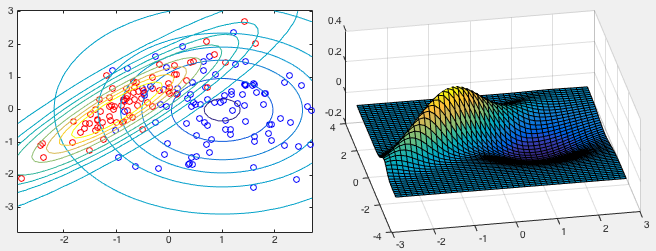
Three classification results are shown in the figure below corresponding to different values used in the kernel function. On the left, the 2-D space is partitioned into red and blue regions corresponding to the two classes based on the sign function of ${\bf m}_{f_*\vert y}$; on the right, the 3-D distribution plots of $\sigma({\bf m}_{f_*\vert y})$ representing the estimated probability for ${\bf x}_*$ to belong to either class (not normalized) is shown, to be compared with the original Gaussian distributions from which the traning samples were drawn.

We see that wherever there is evidence represented by the training samples of either class in red or blue, there are high probabilities for the neighboring points to belong to either $C_1$ or $C_0$ represented by the positive or negative peaks in the 3-D plots. Data points far away from any evidence will have low probability to belong to either class.

We make the following observations for three different values of the parameter $\alpha$ in SE:

• $\alpha=0.4$ (top row), the space is partitioned into three regions, with 20 out of 180 training points misclassified. The estimated distribution is smooth.
• $\alpha=0.2$ (middle row), the space is fragmented into several more pieces for the two classes (blue islands inside the red region and vice versa), with 5 out of the 180 training points misclassified. The estimated distribution is jagged.
• $\alpha=0.03$ (bottom row), the space is partitioned into still more pieces, with all 180 training points correctly classified. The estimated distribution is spiky.

Although the error rate is lowest when $\alpha$ is small, the classificatioin result is not necessarily the best as it may well be an overfitting of the noisy data. We conclude that by adjusting parameter $\alpha$, we can make proper tradeoff between error rate and overfitting.