Gaussian Process Regression

The Gaussian process regression (GPR) is yet another regression method that fits a regression function $f({\bf x})$ to the data samples in the given training set. Different from all previously considered algorithms that treat $f({\bf x})$ as a deterministic function with an explicitly specified form, the GPR treats the regression function $f({\bf x})$ as a stochastic process called Gaussian process (GP), i.e., the function value $f({\bf x})$ at any point ${\bf x}$ is assumed to be a random variable with a Gaussian distribution.

The joint probability distribution of the vector function ${\bf f}({\bf X})=[f({\bf x}_1),\dots,f({\bf x}_N)]^T$ for all $N$ i.i.d. samples in the training set ${\bf X}$ is also Gaussian:

$$p({\bf f}\vert{\bf X})={\cal N}({\bf m}_f,\;{\bf\Sigma}_f) ={\cal N}({\bf0},\;{\bf\Sigma}_f)$$ (251)

where, for convenience and without loss of generality, we have assumed a zero mean ${\bf m}_f={\bf0}$. The ultimate goal is to estimate the regression function $f({\bf x})$ in terms of its Gaussian pdf $p({\bf f}\vert{\bf X})$.

We also assume ${\bf y}={\bf f}({\bf x})+{\bf n}$ as the labeling of ${\bf X}$ in the training set is contaminatd by noise ${\bf n}$, with a zero-mean normal pdf

$$p({\bf n})={\cal N}({\bf n},\,{\bf0},\,\sigma_n^2{\bf I})$$ (252)

where the diagonal covariance matrix $\sigma_n^2{\bf I}$ is based on the assumption that all components of ${\bf n}$ are independent of each other. We further assume noise ${\bf n}$ is independent of ${\bf f}$ with $Cov({\bf y},{\bf n})={\bf0}$. Now ${\bf y}={\bf f}({\bf X})+{\bf n}={\bf f}+{\bf n}$, as the sum of two zero-mean Gaussian variables, is also a zero mean Gaussian process.

The unknown covariance matrix ${\bf\Sigma}_f$ can be constructed based on the desired smoothness of the regression function $f({\bf x})$, in the sense that any two function values $f({\bf x}_m)$ and $f({\bf x}_n)$ are likely to be more correlated if the distance $\vert\vert{\bf x}_m-{\bf x}_n\vert\vert$ between the two corresponding points is small, but less so if the distance is large. Such a covariance can be modeled by a squared exponential (SE) kernel function:

$$Cov(f({\bf x}_m),f({\bf x}_n)) =\exp\left(-\frac{1}{a^2}\vert\ver... ...{\bf x}_n\vert\vert^2\right) =k({\bf x}_m,\,{\bf x}_n)=k({\bf x}_n,\,{\bf x}_m)$$ (253)

where $k({\bf x}_m,\,{\bf x}_n)$ is a kernel function of ${\bf x}_m$ and ${\bf x}_n$. This SE function may take any value between 1 when $\vert\vert{\bf x}_m-{\bf x}_n\vert\vert=0$ and $f({\bf x}_m)=f({\bf x}_n)$ are maximally correlated, and 0 when $\vert\vert{\bf x}_m-{\bf x}_n\vert\vert=\infty$ and $f({\bf x}_m)$ and $f({\bf x}_n)$ are minimally correlated. We therefore see that the SE so constructed mimics the covariance of a smooth function $f({\bf x})$.

The smoothness of the function $f({\bf x})$ plays a very important role as it determines whether the function overfits or underfits the sample points in the training data. If the function is not smooth enough, it may overfit as it may overly affected by some noisy samples; on the other hand, if the function is too smooth, it may underfit as it may not follow the training samples closely enough.

The smoothness of the regression function can be controlled by the hyperparameter $\alpha$ in Eq. (253). Consider two extreme cases. If $a\rightarrow\infty$, i.e., the value of the SE approaches 1, then $f({\bf x}_m)$ and $f({\bf x}_n)$ are highly correlated and $f({\bf x})$ is smooth; on the other hand, if $a\rightarrow 0$, i.e., SE approaches 0, then $f({\bf x}_m)$ and $f({\bf x}_n)$ are not correlated and $f({\bf x})$ is not smooth. Therefore by adjusting the value of $a$, a proper tradeoff between overfitting and underfitting can be made.

Given the covariance $Cov(f({\bf x}_m),f({\bf x}_n))=k({\bf x}_m,{\bf x}_n)$ of function values at two different sample points ${\bf x}_m$ and ${\bf x}_n$, we can represent the covariance matrix of the prior $p({\bf f}\vert{\bf X})$ as

$${\bf\Sigma}_f=Cov({\bf f},{\bf f}) =\left[\begin{array}{ccc} k({\... ...cdots & k({\bf x}_N,\,{\bf x}_N) \end{array}\right] =K({\bf X},{\bf X})={\bf K}$$ (254)

Note that the value of all diagonal components are the same $k({\bf x}_n,{\bf x}_n)=1\;(n=1,\cdots,N)$; and the greater the distance $\vert\vert{\bf x}_m-{\bf x}_n\vert\vert$, the farther away the component $k({\bf x}_m,{\bf x}_n)$ is from the diagonal, and the lower value it takes.

Once the conditional probability $p({\bf f}\vert{\bf X})={\cal N}({\bf0},{\bf\Sigma}_f)$ is estimated based on the training set ${\bf X}=[{\bf x},\cdots,{\bf x}_N]$, we can get the mean and covariance of ${\bf f}_*={\bf f}({\bf X}_*)$ of a test dataset ${\bf X}_*=[{\bf x}_{1*},\cdots,{\bf x}_{M*}]$ containing $M$ unlabeled test samples. As both ${\bf f}_*$ and ${\bf f}$ are the same zero-mean Gaussian process, their joint distribution (given ${\bf X}_*$ as well as ${\bf X}$) is also a zero-mean Gaussian:

$$p\left(\left[\begin{array}{c}{\bf f}\\ {\bf f}_*\end{array}\right] \bigg\vert {\bf X},{\bf X}_*\right) = {\cal N}\left( \left[\begin{array}{c}{\bf f}\\ {\bf f}_*\end{arra... ...igma}_{ff_*}\\ {\bf\Sigma}_{f_*f} & {\bf\Sigma}_{f_*}\end{array}\right]\right)$$

$$= {\cal N}\left( \left[\begin{array}{c}{\bf f}\\ {\bf f}_*\end{arra... ... {\bf K} & {\bf K}_* \\ {\bf K}_*^T & {\bf K}_{**} \end{array} \right] \right)$$ (255)

where

$$\left\{\begin{array}{l} {\bf\Sigma}_{ff_*}=Cov({\bf f},{\bf f}_*)... ...({\bf f}_*,{\bf f}_*)=K({\bf X}_*,{\bf X}_*)={\bf K}_{**}\\ \end{array}\right.$$ (256)

can all be constructed based on the SE function, same as how $K({\bf X},{\bf X})={\bf K}$ is constructed.

Having found the joint pdf $p({\bf f},{\bf f}_*\vert{\bf X},{\bf X}_*)$ of both ${\bf f}$ and ${\bf f}_*$ in Eq. (255), we can further find the conditional distribution $p({\bf f}_*\vert{\bf f},{\bf X},{\bf X}_*)$ of ${\bf f}_*$ given ${\bf f}$ (as well as ${\bf X}$ and ${\bf X}_*$), based on the properties of the Gaussian distributions discussed in the Appendices:

$$p({\bf f}_*\vert{\bf f},{\bf X},{\bf X}_*) ={\cal N}({\bf m}_{(f_*\vert f)},{\bf\Sigma}_{(f_*\vert f)})$$ (257)

with the mean and covariance

$$\left\{ \begin{array}{lcl} {\bf m}_{(f_*\vert f)}&=&\E[ {\bf f}_*... ...\vert{\bf f})={\bf K}_{**}-{\bf K}_*^T {\bf K}^{-1}{\bf K}_* \end{array}\right.$$ (258)

Similarly, we can also find the joint distribution of ${\bf f}_*$ and ${\bf y}={\bf f}+{\bf r}$, both of which are zero-mean Gaussian:

$$p({\bf y},{\bf f}_*\vert{\bf X},{\bf X}_*)={\cal N}\left( \left[\... ...igma}_{yf_*}\\ {\bf\Sigma}_{f_*y} & {\bf\Sigma}_{f_*}\end{array}\right]\right)$$ (259)

where

$${\bf\Sigma}_y = Cov({\bf y},{\bf y})=Cov({\bf f}+{\bf n},{\bf f}+{\bf n}) =Cov({\bf f},{\bf f})+2\,Cov({\bf f},{\bf n})+Cov({\bf n},{\bf n})$$

$$= Cov({\bf f},{\bf f})+Cov({\bf r},{\bf r})={\bf\Sigma}_f+{\bf\Sigma}_n ={\bf K}+\sigma_n^2{\bf I}$$

$${\bf\Sigma}_{yf_*} = Cov({\bf y},{\bf f}_*) =Cov({\bf f}+{\bf n},{\bf f}_*) =Cov({\bf f},{\bf f}_*)+Cov({\bf f},{\bf n}_*)$$

$$= Cov({\bf f},{\bf f}_*)={\bf\Sigma}_{ff_*}={\bf K}_*$$ (260)

where $Cov({\bf f},{\bf n})=Cov({\bf f}_*,{\bf n})={\bf0}$. Now we have

$$Cov\left[ \begin{array}{c} {\bf y} \\ {\bf f}_* \end{array} \righ... ...sigma_n^2{\bf I} & {\bf K}_* \\ {\bf K}^T_* & {\bf K}_{**} \end{array} \right]$$ (261)

We can now further get the desired conditional distribution of ${\bf f}_*$ given ${\bf X}_*$ as well as the training set ${\cal D}=\{{\bf X},\,{\bf y}\}$:

$$p({\bf f}_*\vert{\bf X}_*,{\cal D})=p({\bf f}_*\vert{\bf X}_*,{\bf X},{\bf y}) ={\cal N}({\bf m}_{(f_*)},{\bf\Sigma}_{(f_*)})$$ (262)

with the mean and covariance

$$\left\{ \begin{array}{lcl} {\bf m}_{(f_*)}&=&\E[ {\bf f}_*\vert{\... ...K}_*^T \left({\bf K}+\sigma_n^2{\bf I}\right)^{-1} {\bf K}_* \end{array}\right.$$ (263)

We see that these expressions are the same as those in Eq. (184) previously obtained by Bayesian linear regression, i.e., the same results can be derived by two very different methods.

In the special noise-free case of ${\bf n}={\bf0}$ (with zero mean and zero covariance $\sigma_n^2=0$), we have ${\bf y}={\bf f}+{\bf n}={\bf f}$, and the mean and covariance in Eq. (263) become the same as Eq. (258), and Eqs. (262) and (257) become the same:

$$p({\bf f}_*\vert{\bf X}_*,{\bf X},{\bf y}) =p({\bf f}_*\vert{\bf X}_*,{\bf X},{\bf f})$$ (264)

The Matlab code below for the Gaussian process regression algorithm, takes the training set ${\cal D}=\{ {\bf X},{\bf y}\}$, the test samples in ${\bf X}_*$, and the variance $\sigma^2_n$ of the noise as the input, and generates as the output the posterior $p({\bf f}_*\vert{\cal D},{\bf X}_*)$, in terms of its mean as the GPR regression function, and its covariance matrix, of which the variances on the diagonal represent the confidence or certainty of the regression.

function [fmean fcov]=GPR(X,y,Xstar,sigmaN)   % given training set D={X,y}, test sample Xstar
                                              % find regression function fmean and covariance
    Sy=Kernel(X,X)+sigmaN^2*eye(length(X));   % Covariance of training samples
    Syf=Kernel(X,Xstar);                      % Covariance of training and test samples
    Sf=Kernel(Xstar,Xstar);                   % Covariance of test samples
    fmean=Syf'*inv(Sy)*y;                     % mean of posterior as the regression function
    fcov=Sf-Syf'*inv(Sy)*Syf;                 % covariance of posterior
end

The follwoing code is for a function that generates the squared exponential kernel matrix based on two sets of data samples in X1 and X2:

function K=Kernel(X1,X2)
    a=1;            % parameter that controls smoothness of f(x)
    m=length(X1);
    n=length(X2);
    K=zeros(m,n);       
    for i=1:m
        for j=1:n
            d=norm(X1(:,i)-X2(:,j));
            K(i,j)=exp(-(d/a)^2);
        end
    end
end

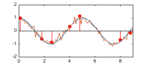
Example:

A sinusoidal function $f(x)=\cos(2\pi f x)\;(f=0.2)$ contaminated by Gaussian noise $e$ with $p(r)={\cal N}(0,\,\sigma_r^2)\;(\sigma_r=0.2)$ is sampled at $N=7$ random positions over the duration of the function $(0,\;0)$. These samples form the training dataset ${\cal D}=\{ (x_n, y_n)\,(n=1,\cdots,N)\}$.

Then the method of GPR is used to estimate the mean and variance of $f_{i*}=f(x_{i*})$ at 91 test points $x_{i*}$, evenly distributed over the duration of the function between the limits $x_{min}=0$ and $x_{max}=9$,

The 8 panels of the figure below show the estimated mean $\E[f_*]$, and the variance $\pm \Var[f_*]$, both above and below the mean, to form a region of uncertainty of the estimates. The wider the region, the more uncertain the results are (less confidence).

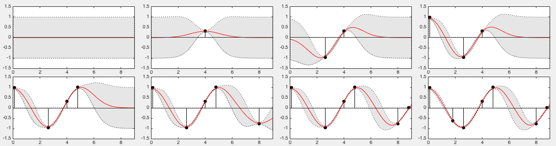
The top left panel represents the prior probability $p(f_*\vert x_*)$ of the estimated model output $f_*=\hat{y}_*$ at point $x_*$ with no knowledge based on the training set ${\bf x}$ ($N=0$ training samples), which is assumed to have zero-mean $\E[f_*]=0$ and unity variance $\Var[f(x_*)]=k(x_*, x_*)=1$. The subsequent seven panels show the mean and variance of the posterior $p(f_*=\hat{y}_*\vert x_*,{\cal D})$ based on $N=1,\cdots,7$ training samples in the training set${\cal D}$. Note that wherever a training sample $x$ becomes available, the estimated mean $\mu_{f_*\vert y}$ is modified to be close to the true function value $f(x)$, and the variance of the posterior around $x$ is reduced, indicating the uncertainty of the estimate is reduced, or the confidence is much increased. When all $N=7$ training samples are used, the general shape of the original function is reasonably reconstructed.

The 8 panels in the figure below show 12 sample curves drawn from each posterior $p(f_*\vert{\bf x}_*,{\cal D})$. They can be treated as different interpolations for the $N$ observed samples in training set ${\cal D}$, and any of them can be used to predict the outputs $y_*$ at any input points $x_*$. The mean of these samples shown as the red curve is simply the same as $\E[f_*]$ shown in the previous figure.

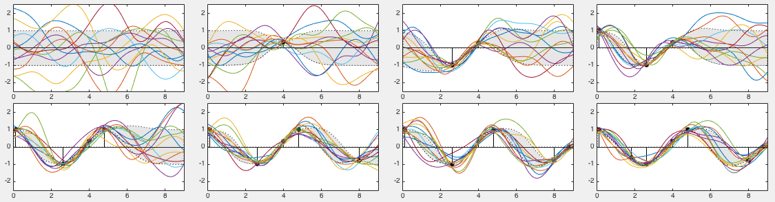
We see that wherever a training sample $f(x)$ is available at $x$, the variance and thereby the width of the region of uncertainty is reduced, and correspondingly the sample curves in the neighborhood of $x$ are more tightly distributed. Specifically, we see that the sample curves drawn from the prior in the top left panel are very loosely distributed, while those samples drawn from the posterior obtained based on all $N=7$ training points in the bottom right panel are relatively tightly distributed. In particular, note that due to lack of training data in the interval $5<x<8$, the region of uncertainty is significantly wider than else where, and the sample curves are much more loosely located.

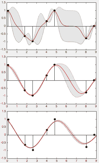
The parameter $\alpha$ of the kernel function plays an important role in the GPR results, as shown in the three panels in the figure below, corresponding respectively to $a$ values of 0.5, 1.5, and 3.0. When $a$ is too small (top panel), the model may overfit the data, as the regression function fits the training samples well but it not smooth and it does not interpolate regions between the training samples well (with large variance); one the other hand, when $a$ is too large (bottom panel), the model may underfit the data, as the regression curve is smooth, but it does not fit the training samples well. We therefore see that we need to choose the value of $a$ carefully for a proper tradeoff between overfitting and underfitting (middle panel).