Quasi-Newton Methods

As we have seen above, Newton's methods can be used to solve both nonlinear systems to find roots of a set of simultaneous equations, and optimization problems to minimize a scalar-valued objective function based on the iterations of the same form. Specifically,

• Solving equations ${\bf f}({\bf x})={\bf0}$:

  $${\bf x}_{n+1}={\bf x}_n-{\bf J}({\bf x}_n)^{-1}{\bf f}({\bf x}_n) ={\bf x}_n-{\bf J}_n^{-1}{\bf f}_n$$ (78)

  where ${\bf J}_n={\bf J}({\bf x}_n)$ is the Jacobian matrix of ${\bf f}({\bf x}_n)$,
• Minimizing $f({\bf x})$:

  $${\bf x}_{n+1}={\bf x}_n-{\bf H}({\bf x}_n)^{-1}{\bf g}({\bf x}_n) ={\bf x}_n-{\bf H}_n^{-1}{\bf g}_n$$ (79)

  where ${\bf g}_n={\bf g}({\bf x}_n)$ and ${\bf H}_n={\bf H}({\bf x}_n)$ are the gradient vector and Hessian matrix of $f({\bf x})$ at ${\bf x}_n$, respectively.

If the Jacobian ${\bf J}({\bf x})$ or the Hessian matrix ${\bf H}({\bf x})$ is not available, or if it is too computationally costly to calculate its inverse (with complexity $O(N^3)$), the quasi-Newton methods can be used to approximate the Hessian matrix or its inverse based only on the first order derivative, the gradient ${\bf g}$ of $f({\bf x})$ (with complexity $O(N^2)$), similar to Broyden's method previously considered.

In the following, we consider the minimization of a function $f({\bf x})$. Its Taylor expansion around point ${\bf x}_{n+1}$ is

$$f({\bf x})=f({\bf x}_{n+1})+({\bf x}-{\bf x}_{n+1})^T {\bf g}_{n+... ...H}_{n+1} ({\bf x}-{\bf x}_{n+1})+O(\vert\vert{\bf x}-{\bf x}_{n+1}\vert\vert^3)$$ (80)

Taking derivetive with respect to ${\bf x}$, we get

$$\frac{d}{d{\bf x}}f({\bf x})={\bf g}({\bf x}) ={\bf g}_{n+1}+{\bf H}_{n+1} ({\bf x}-{\bf x}_{n+1}) +O(\vert\vert{\bf x}-{\bf x}_{n+1}\vert\vert^2)$$ (81)

Evaluating at ${\bf x}={\bf x}_n$, we have ${\bf g}({\bf x}_n)={\bf g}_n$, and the above can be written as

$${\bf g}_{n+1}-{\bf g}_n = {\bf H}_{n+1}({\bf x}_{n+1}-{\bf x}_n) +O(\vert\vert{\bf x}_{n+1}-{\bf x}_n\vert\vert^2)$$

$$= {\bf B}_{n+1}({\bf x}_{n+1}-{\bf x}_n)$$ (82)

where matrix ${\bf B}_n$ is the secant approximation of the Hessian matrix ${\bf H}_n$, and the last eqality is called the secant equation. For convenience, we further define:

$${\bf s}_n={\bf x}_{n+1}-{\bf x}_n,\;\;\;\;\;\; {\bf y}_n={\bf g}_{n+1}-{\bf g}_n$$ (83)

so that the equation above can be written as

$${\bf B}_{n+1}{\bf s}_n={\bf y}_n,\;\;\;\;\; \;\;\;\;\; {\bf B}_{n+1}^{-1}{\bf y}_n={\bf s}_n$$ (84)

This is the quasi-Newton equation, which is the secant condition that must be satisfied by matrix ${\bf B}_n$, or its inverse ${\bf B}_n^{-1}$, in any of the quasi-Newton algorithms, all taking the follow general steps:

1. Initialize ${\bf x}_0$ and ${\bf B}_0$, set $n=0$;
2. Compute gradient ${\bf g}_n$ and the search direction ${\bf d}_n=-{\bf B}_n^{-1}{\bf g}_n$;
3. Get ${\bf x}_{n+1}={\bf x}_n+\delta{\bf d}_n$ with step size $\delta$ satisfying the Wolfe conditions.
4. update ${\bf B}_{n+1}={\bf B}_n+\Delta{\bf B}_n$ or ${\bf B}_{n+1}^{-1}={\bf B}_n^{-1}+\Delta{\bf B}_n^{-1}$, that satisfies the quasi-Newton equation;
5. If termination condition is not satisfied, $n=n+1$, go back to second step.

For this iteration to converge to a local minimum of $f({\bf x})$, ${\bf B}_n$ must be positive definite matrix, same as the Hessian matrix ${\bf H}$ it approximates. Specially, if ${\bf B}_n={\bf I}$, then ${\bf d}_n=-{\bf g}_n$, the algorithm becomes the gradient descent method; also, if ${\bf B}_n={\bf H}_n$ is the Hessian matrix, then the algorithm becomes the Newton's method.

In a quasi-Newton method, we can choose to update either ${\bf B}_n$ or its inverse ${\bf B}_n^{-1}$ based on one of the two forms of the quasi-Newton equation. We note that there is a dual relationship between the two ways to update, i.e., by swapping ${\bf y}_n$ and ${\bf s}_m$, an update formula for ${\bf B}_n$ can be directly applied to its inverse and vice versa.

• The Symmetric Rank 1 (SR1) Algorithm

  Here matrix ${\bf B}_n$ is updated by an additional term:

  $${\bf B}_{n+1}={\bf B}_n+{\bf uu}^T$$ (85)

  where ${\bf u}$ a vector and ${\bf uu}^T$ is a matrix of rank 1. Imposing the secant condition, we get

  $${\bf B}_{n+1}{\bf s}_n ={\bf B}_n{\bf s}_n+{\bf uu}^T{\bf s}_n={\bf y}_n, \;\;\;\; \;\;\;\;\; {\bf u}({\bf u}^T{\bf s}_n)={\bf y}_n-{\bf B}_n{\bf s}_n$$ (86)

  This equation indicats ${\bf u}$ is in the same direction as ${\bf w}={\bf y}_n-{\bf B}_n{\bf s}_n$, and can therefore be written as ${\bf u}=c {\bf w}$. Substituting this back we get

  $${\bf u}{\bf u}^T{\bf s}_n=c^2{\bf w}{\bf w}^T{\bf s}_n={\bf w}$$ (87)

  Solving this we get $c =1/({\bf w}^T {\bf s}_n)^{1/2}$,

  $${\bf u}=c{\bf w}=\frac{{\bf y}_n-{\bf B}_n{\bf s}_n}{({\bf w}^T{\... ...bf y}_n-{\bf B}_n{\bf s}_n}{( ({\bf y}_n-{\bf B}_n{\bf s}_n)^T{\bf s}_n)^{1/2}}$$ (88)

  and the iteration of ${\bf B}_n$ becomes

  $${\bf B}_{n+1}={\bf B}_n+{\bf uu}^T ={\bf B}_n +\frac{ ({\bf y}_n-... ...\bf y}_n-{\bf B}_n{\bf s}_n)^T } { ({\bf y}_n-{\bf B}_n{\bf s}_n)^T {\bf s}_n }$$ (89)

  Applying the Sherman-Morrison formula, we can further get the inverse ${\bf B}_{n+1}$:
  

  $${\bf B}_{n+1}^{-1} = \left( {\bf B}_n+{\bf uu}^T \right)^{-1} ={\bf B}_n^{-1}-\frac{ {\bf B}_n^{-1}{\bf uu}^T{\bf B}_n^{-1}}{1+{\bf u}^T{\bf B}_n^{-1}{\bf u}}$$

  $$= {\bf B}_n^{-1} +\frac{ ({\bf s}_n-{\bf B}_n^{-1}{\bf y}_n)({\bf s... ...\bf B}_n^{-1}{\bf y}_n)^T } { ({\bf s}_n-{\bf B}_n^{-1}{\bf y}_n)^T {\bf y}_n }$$ (90)

  
  We note that this equation is dual to the previous one, and it can also be obtained based on the duality between the secant conditions for ${\bf B}_n$ and ${\bf B}_n^{-1}$. Specifically, same as above, we impose the secant condition for the inverse ${\bf B}_{n+1}^{-1}$ of the following form

  $${\bf B}_{n+1}^{-1}={\bf B}_n^{-1}+{\bf uu}^T$$ (91)

  and get

  $${\bf B}_{n+1}^{-1}{\bf y}_n ={\bf B}_n^{-1}{\bf y}_n+{\bf uu}^T{\bf y}_n={\bf s}_n,$$ (92)

  Then by repeating the same process above, we get the same update formula for ${\bf B}_n^{-1}$.

  This is the formula for directly updating ${\bf B}_n^{-1}$. For the iteration to converge to a local minimum, matrix ${\bf B}_{n+1}^{-1}$ needs to be positive definite as well as ${\bf B}_n^{-1}$, we therefore require

  $${\bf w}^T{\bf y}_n=({\bf s}_n-{\bf B}_n^{-1}{\bf y}_n)^T {\bf y}_n ={\bf s}_n^T{\bf y}_n -{\bf y}_n^T {\bf B}_n^{-1}{\bf y}_n >0$$ (93)

  It may be difficult to maintain this requirement through out the iteration. This problem can be avoided in the following DFP and BFGS methods.

• The BFGS (Broyden-Fletcher-Goldfarb-Shanno) algorithm

  This is a rank 2 algorithm in which matrix ${\bf B}_n$ is updated by two rank-1 terms:

  $${\bf B}_{n+1}={\bf B}_n+\alpha{\bf uu}^T+\beta{\bf vv}^T$$ (94)

  Imposing the secant condition for ${\bf B}_n$, we get

  $${\bf B}_{n+1} {\bf s}_n =({\bf B}_n+\alpha{\bf uu}^T+\beta{\bf vv... ...n+{\bf u}(\alpha{\bf u}^T{\bf s}_n) +{\bf v}(\beta{\bf v}^T{\bf s}_n)={\bf y}_n$$ (95)

  or

  $${\bf u}(\alpha{\bf u}^T{\bf s}_n) +{\bf v}(\beta{\bf v}^T{\bf s}_n)={\bf y}_n-{\bf B}_n{\bf s}_n$$ (96)

  which can be satisfied if we let

  $${\bf u}={\bf y}_n,\;\;\;\;\;\;\alpha=\frac{1}{{\bf s}_n^T{\bf y}_... ...\; \beta=-\frac{1}{{\bf v}^T{\bf s}_n}=-\frac{1}{{\bf s}_n^T{\bf B}_n{\bf s}_n}$$ (97)

  Substituting these into ${\bf B}_{n+1}={\bf B}_n+\alpha{\bf uu}^T+\beta{\bf vv}^T$ we get

  $${\bf B}_{n+1}={\bf B}_n+\alpha{\bf uu}^T+\beta{\bf vv}^T ={\bf B}... ...} -\frac{{\bf B}_n{\bf s}_n{\bf s}_n^T{\bf B}_n}{{\bf s}_n^T{\bf B}_n{\bf s}_n}$$ (98)

  Given this update formula for ${\bf B}_n$, we can further find its inverse ${\bf B}_n^{-1}$ and then the search direction ${\bf d}_n=-{\bf B}_n^{-1}{\bf g}_n$.

  Alternatively, given ${\bf B}_n$, we can further derive an update formula directly for the inverse matrix ${\bf B}_n^{-1}$, so that the search direction ${\bf d}_n$ can be obtained without carrying out the inversion computation. Specifically, we first define ${\bf U}=[{\bf u}_1\;{\bf u}_2]$ and ${\bf V}=[{\bf v}_1\;{\bf v}_2]$, where

  $${\bf u}_1={\bf v}_1=\frac{{\bf y}_n}{({\bf s}_n^T{\bf y}_n)^{1/2}... ...}_2=-{\bf v}_2=\frac{{\bf B}_n{\bf s}_n}{({\bf s}_n^T{\bf B}_n{\bf s}_n)^{1/2}}$$ (99)

  so that the expression above can be written as:

  $${\bf B}_{n+1}={\bf B}_n+{\bf u}_1{\bf v}_1^T+{\bf u}_2{\bf v}_2^T =({\bf B}_n+{\bf UV}^T)^{-1}$$ (100)

  and then apply the Sherman-Morrison formula, to get:
  

  $${\bf B}_{n+1}^{-1} = ({\bf B}_n+{\bf UV}^T)^{-1} ={\bf B}_n^{-1}-{\bf B}_n^{-1}{\bf U}({\bf I}+{\bf V}^T{\bf B}_n^{-1}{\bf U})^{-1}{\bf V}^T{\bf B}_n^{-1}$$

  $$= {\bf B}_n^{-1}-{\bf B}_n^{-1}{\bf U}{\bf C}^{-1}{\bf V}^T{\bf B}_... ...{-1}[{\bf u}_1\;{\bf u}_2]{\bf C}^{-1} ({\bf B}_n^{-1}[{\bf v}_1\;{\bf v}_2])^T$$ (101)

  
  where we have defined

  $${\bf C}=\left[\begin{array}{cc}c_{11} & c_{12}\\ c_{21} & c_{22}\... ...1}{\bf U} ={\bf I}+[{\bf v}_1\;{\bf v}_2]^T{\bf B}^{-1}_n[{\bf u}_1\;{\bf u}_2]$$ (102)

  with

  $$c_{11}=1+{\bf v}^T_1{\bf B}_n^{-1}{\bf u}_1 =1+\frac{{\bf y}^T_n{\bf B}_n^{-1}{\bf y}_n}{{\bf s}_n^T{\bf y}_n}$$ (103)

  $$c_{22}=1+{\bf v}_2{\bf B}_n^{-1}{\bf u}_2 =1-\frac{{\bf s}_n^T{\bf B}_n{\bf B}_n^{-1}{\bf B}_n{\bf s}_n}{{\bf s}_n^T{\bf B}_n{\bf s}_n} =0$$ (104)

  $$c_{12}={\bf v}_1^T{\bf B}_n^{-1}{\bf u}_2 =\frac{{\bf y}_n^T{\bf ... ... } =\frac{({\bf s}_n^T{\bf y}_n)^{1/2}}{({\bf s}_n^T{\bf B}_n{\bf s}_n)^{1/2} }$$ (105)

  $$c_{21}={\bf v}_2^T{\bf B}_n^{-1}{\bf u}_1=-c_{12}$$ (106)

  $${\bf C}=\left[\begin{array}{cc}c_{11} & c_{12}\\ -c_{12} & 0\end{... ...t[\begin{array}{cc}0 & -1/c_{12}\\ 1/c_{12} & c_{11}/c_{12}^2\end{array}\right]$$ (107)

  Substituting this ${\bf C}^{-1}$ into the expression for ${\bf B}_{n+1}^{-1}$, we get:
  

  $${\bf B}_{n+1}^{-1} = {\bf B}_n^{-1}-[{\bf B}_n^{-1}{\bf u}_1\;{\bf B}_n^{-1}{\bf u}_2]... ...c_{12}^2\end{array}\right] [{\bf B}_n^{-1}{\bf v}_1\;{\bf B}_n^{-1}{\bf v}_2]^T$$

  $$= {\bf B}_n^{-1}-\frac{1}{c_{12}} [{\bf B}_n^{-1}{\bf u}_2{\bf v}_1... ...^{-1}] -\frac{c_{11}}{c_{12}^2}{\bf B}_n^{-1}{\bf u}_2{\bf v}_2^T{\bf B}_n^{-1}$$ (108)

  
  where

  $$\frac{1}{c_{12}}{\bf B}_n^{-1}{\bf u}_2{\bf v}_1^T{\bf B}_n^{-1} ... ...{\bf B}_n^{-1} =\frac{{\bf s}_n{\bf y}_n^T{\bf B}_n^{-1}}{{\bf s}_n^T{\bf y}_n}$$ (109)

  $$-\frac{1}{c_{12}}{\bf B}_n^{-1}{\bf u}_1{\bf v}_2^T{\bf B}_n^{-1}... ...{\bf B}_n^{-1} =\frac{{\bf B}_n^{-1}{\bf y}_n{\bf s}_n^T}{{\bf s}_n^T{\bf y}_n}$$ (110)

  
  

  $$\frac{c_{11}}{c_{12}^2}{\bf B}_n^{-1}{\bf u}_2{\bf v}_2^T{\bf B}_n^{-1} = -\left(1+\frac{{\bf y}^T_n{\bf B}_n^{-1}{\bf y}_n}{{\bf s}_n^T{\b... ...ac{{\bf s}_n^T {\bf B}_n}{({\bf s}_n^T{\bf B}_n{\bf s}_n)^{1/2}} {\bf B}_n^{-1}$$

  $$= -\left(1+\frac{{\bf y}^T_n{\bf B}_n^{-1}{\bf y}_n}{{\bf s}_n^T{\bf y}_n}\right) \frac{{\bf s}_n{\bf s}_n^T}{{\bf s}_n^T{\bf y}_n}$$ (111)

  
  Substituting these three terms back into Eq. (108), we get the update formula for ${\bf B}_n^{-1}$:

  $${\bf B}_{n+1}^{-1}= {\bf B}_n^{-1}-\frac{{\bf B}_n^{-1}{\bf y}_n{... ...{{\bf s}_n^T{\bf y}_n}\right) \frac{{\bf s}_n{\bf s}_n^T}{{\bf s}_n^T{\bf y}_n}$$ (112)

  In summary, ${\bf B}_{n+1}^{-1}$ can be found by either Eq. (98) for ${\bf B}_{n+1}$ followed by an additional inversion operation, or Eq. (112) directly for ${\bf B}_{n+1}^{-1}$. The results obtained by these methods are equivalent.

• The DFP (Davidon-Fletcher-Powell) Algorithm

  Same as the BFGS algorithm, the DFP algorithm is also a rank 2 algorithm, where instead of ${\bf B}_n$, the inverse matrix ${\bf B}^{-1}_n$ is updated by two rank-1 terms:

  $${\bf B}^{-1}_{n+1}={\bf B}_n^{-1}+\alpha{\bf uu}^T+\beta{\bf vv}^T$$ (113)

  where $\alpha$ and $\beta$ are real scalars, ${\bf u}$ and ${\bf v}$ are vectors. Imposing the secant condition for the inverse of ${\bf B}_n$, we get

  $${\bf B}_{n+1}^{-1} {\bf y}_n =({\bf B}_n^{-1}+\alpha{\bf uu}^T+\b... ...n+{\bf u}(\alpha{\bf u}^T{\bf y}_n) +{\bf v}(\beta{\bf v}^T{\bf y}_n)={\bf s}_n$$ (114)

  or

  $${\bf u}(\alpha{\bf u}^T{\bf y}_n) +{\bf v}(\beta{\bf v}^T{\bf y}_n)={\bf s}_n-{\bf B}_n^{-1}{\bf y}_n$$ (115)

  which can be satisfied if we let

  $${\bf u}={\bf s}_n,\;\;\;\;\;\;\alpha=\frac{1}{{\bf s}^T{\bf y}_n}... ...eta=-\frac{1}{{\bf v}^T{\bf y}_n}=-\frac{1}{{\bf y}_n^T{\bf B}_n^{-1}{\bf y}_n}$$ (116)

  Substituting these into ${\bf B}^{-1}_{n+1}={\bf B}^{-1}_n+\alpha{\bf uu}^T+\beta{\bf vv}^T$ we get

  $${\bf B}^{-1}_{n+1}={\bf B}^{-1}_n+\alpha{\bf uu}^T+\beta{\bf vv}^... ...}_n^{-1}{\bf y}_n{\bf y}_n^T{\bf B}_n^{-1}}{{\bf y}_n^T{\bf B}_n^{-1}{\bf y}_n}$$ (117)

  Following the same procedure used for the BFGS method, we can also obtain the update formular of matrix ${\bf B}_n$ for the DFP method:

  $${\bf B}_{n+1}= {\bf B}_n-\frac{{\bf B}_n{\bf s}_n{\bf y}_n^T+{\bf... ...{{\bf y}_n^T{\bf s}_n}\right) \frac{{\bf y}_n{\bf y}_n^T}{{\bf y}_n^T{\bf s}_n}$$ (118)

  We note that Eqs. (117) and (98) form a duality pair, and Eqs. (118) and (112) form another duality pair. In other words, the BFGS and FDP methods are dual of each other.

In both the DFP and BFGS methods, matrix ${\bf B}_n^{-1}$, as well as ${\bf B}_n$, must be positive definite, i.e., ${\bf z}^T{\bf B}_n{\bf z} > 0$ must hold for any ${\bf z}\ne{\bf0}$. We now prove that this requirement is satisfied if the curvature condition of the Wolfe conditions is satisfied:

$${\bf g}_{n+1}^T {\bf d}_n \ge c_2\;{\bf g}_n^T {\bf d}_n \;\;\;\;\;\;\; \;\;\;\;\; \left( {\bf g}_{n+1}-c_2\;{\bf g}_n\right)^T {\bf d}_n \ge 0$$ (119)

Replacing the search direction ${\bf d}_n$ by $\delta{\bf d}_n={\bf x}_{n+1}-{\bf x}_n={\bf s}_n$, we get:

$$({\bf g}_{n+1}-c_2{\bf g}_n)^T {\bf s}_n ={\bf g}^T_{n+1}{\bf s}_n-c_2{\bf g}_n^T {\bf s}_n \ge 0$$ (120)

We also have

$${\bf y}_n^T{\bf s}_n=({\bf g}_{n+1}-{\bf g}_n)^T {\bf s}_n ={\bf g}_{n+1}^T{\bf s}_n-{\bf g}_n^T {\bf s}_n$$ (121)

Substracting the first equation from the second, we get

$${\bf y}_n^T{\bf s}_n- ({\bf g}^T_{n+1}{\bf s}_n-c_2{\bf g}_n^T {\bf s}_n) =(c_2-1){\bf g}_n^T{\bf s}_n > 0$$ (122)

The last inequality is due to the fact that ${\bf g}_n^T{\bf s}_n<0$ and $c_2<1$. We therefore have

$${\bf y}_n^T{\bf s}_n\ge {\bf g}^T_{n+1}{\bf s}_n-c_2{\bf g}_n^T {\bf s}_n \ge 0$$ (123)

Given ${\bf y}_n^T{\bf s}_n>0$, we can further prove by induction that both ${\bf B}_{n+1}$ and ${\bf B}_{n+1}^{-1}$ based repectively on the update formulae in Eqs. (98) and (117) are positive definite. We first assume ${\bf B}_0$ and ${\bf B}_n$ are both positive definite, and express ${\bf B}_n$ in terms of its Cholesky decomposition, ${\bf B}_n={\bf LL}^T$. We further define ${\bf a}={\bf L}^T{\bf z}$, ${\bf b}={\bf L}^T{\bf s}$, and get

$${\bf a}^T{\bf a}={\bf z}^T{\bf B}_n{\bf z},\;\;\;\; {\bf b}^T{\bf b}={\bf s}^T{\bf B}_n{\bf s},\;\;\;\; {\bf a}^T{\bf b}={\bf z}^T{\bf B}_n{\bf s}$$ (124)

Now we can show that the sum of the first and third terms of Eq. (112) is positive definite:

$${\bf z}^T\left[ {\bf B}_n-\frac{{\bf B}_n{\bf s}_n{\bf s}_n^T{\bf... ...{\bf s}_n} ={\bf a}^T{\bf a}-\frac{({\bf a}^T{\bf b})^2}{{\bf b}^T{\bf b}}\ge 0$$ (125)

The last step is due to the Cauchy-Schwarz inequality. Also, as ${\bf s}_n^T{\bf y}_n\ge 0$, the second term of Eq. (98) is positive definite

$${\bf z}^T\left(\frac{{\bf s}_n{\bf s}_n^T}{{\bf s}_n^T{\bf y}_n}\right){\bf z}\ge 0$$ (126)

Combining these two results, we get

$${\bf z}^T{\bf B}_{n+1}{\bf z} = {\bf z}^T\left( {\bf B}_n-\frac{{... ... z}^T\left(\frac{{\bf y}_n{\bf y}_n^T}{{\bf s}_n^T{\bf y}_n}\right){\bf z}\ge 0$$ (127)

i.e., ${\bf B}_{n+1}$ based on the update formular Eq. (98) is positive definite. Following the same steps, we can also show that ${\bf B}_{n+1}^{-1}$ based on Eq. (117) is positive definite.

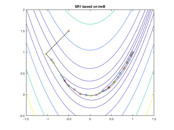
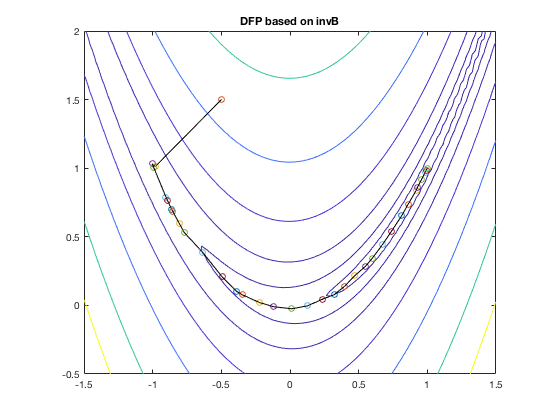
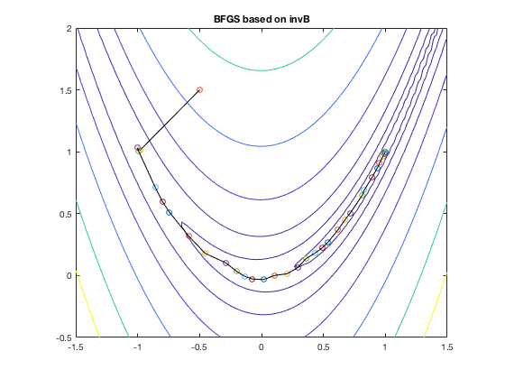
Examples:

The figures below shows the search path of the DFP and BPGS methods when applied to find the minimum of the Rosenbrock function.