Line minimization

In general, in an algorithm for minimizing an objective function $f({\bf x})$, such as Newton's method (Eq. (36)) and the gradient descent method (Eq. (50)), the variable ${\bf x}$ is iteratively updated to gradualy reduce the value of $f({\bf x})$. Specifically, both the search direction ${\bf d}_n$ and the step size $\delta$ in the iteration ${\bf x}_{n+1}={\bf x}_n+\delta_n{\bf d}_n$ need to be determined so that $f({\bf x}_{n+1})$ is maximally reduced.

First we realize that the search direction ${\bf d}_n$ needs to point away from the gradient ${\bf g}_n$ along which $f({\bf x}_n)$ increases most rapidly. In other words, the angle $\theta$ between ${\bf d}_n$ and ${\bf g}_n$ should be greater than $\pi/2$:

$$\theta=\cos^{-1}\left(\frac{{\bf d}_n^T{\bf g}_n}{\vert\vert{\bf ... ...\vert}\right) >\frac{\pi}{2} \;\;\;\;\;{i.e.,}\;\;\;\;\; {\bf d}_n^T{\bf g}_n<0$$ (51)

This condition is indeed satisfied in both the gradient descent method with ${\bf d}_n=-{\bf g}_n$ and Newton's method with ${\bf d}_n=-{\bf H}_n^{-1}{\bf g}_n$:

$${\bf d}_n^T{\bf g}_n=-{\bf g}_n^T{\bf H}_n^{-1}{\bf g}_n <0,\;\;\... ... {\bf d}_n^T{\bf g}_n=-{\bf g}_n^T{\bf g}_n=-\vert\vert{\bf g}_n\vert\vert^2 <0$$ (52)

Here ${\bf H}_n$ is assumed to be positive definite so that a minimum exists.

Next, we need to find the optimal step size $\delta_n$ so that the function value $f({\bf x}_{n+1})=f({\bf x}_n+\delta_n{\bf d}_n)$ is minimized along the search direction ${\bf d}_n$. To do so, we set to zero the derivative of the function with respect to $\delta_n$, the directional derivative along the direction of ${\bf d}_n$, and get the following by chain rule:

$$\frac{d}{d\delta_n} f({\bf x}_{n+1}) =\frac{d}{d\delta_n}f({\bf x... ...\; \frac{d({\bf x}_n+\delta_n{\bf d}_n)}{d\delta_n} ={\bf g}^T_{n+1}{\bf d}_n=0$$ (53)

This result indicates that the gradient ${\bf g}_{n+1}=f'({\bf x}_{n+1})$ at the next point ${\bf x}_{n+1}$ should be perpendicular to the search direction ${\bf d}_n$. In other words, when traversing along ${\bf d}_n$, we should stop at the point ${\bf x}_{n+1}={\bf x}_n+\delta{\bf d}_n$ at which the gradient ${\bf g}_{n+1}$ is perpendicular to ${\bf d}_n$, i.e., it has zero component along ${\bf d}_n$, and the corresponding $\delta$ is the optimal step size.

To find the actual optimal step size $\delta$, we need to solve a 1-D optimization problem while treating $f({\bf x}_{n+1})=f({\bf x}_n+\delta{\bf d}_n)$ as a function of the step size $\delta$ as a variable, and approximate it by the first three terms of its Taylor series at $\delta=0$ (Maclaurin series of function $f(\delta)$):

$$f({\bf x}_{n+1})=f({\bf x}_n+\delta{\bf d}_n)\approx \left[f({\bf... ...}{2}\;\left[\frac{d^2}{d\delta^2}f({\bf x}_n+\delta{\bf d}_n)\right]_{\delta=0}$$ (54)

where

$$\left[f({\bf x}_n+\delta{\bf d}_n)\right]_{\delta=0} = f({\bf x}_n)$$ (55)

$$\left[\frac{d}{d\delta}f({\bf x}_n+\delta{\bf d}_n)\right]_{\delta=0} = \left[{\bf g}({\bf x}_n+\delta{\bf d}_n)^T{\bf d}_n\right]_{\delta=0} ={\bf g}^T_n{\bf d}_n$$ (56)

$$\left[\frac{d^2}{d\delta^2}f({\bf x}_n+\delta{\bf d}_n)\right]_{\delta=0} = \left[\frac{d}{d\delta}{\bf g}({\bf x}_n +\delta{\bf d}_n)^T\righ... ...})\; \frac{d}{d\delta}({\bf x}_n+\delta{\bf d}_n)\right]^T_{\delta=0} {\bf d}_n$$

$$= ({\bf H}_n{\bf d}_n)^T{\bf d}_n={\bf d}^T_n{\bf H}_n{\bf d}_n$$ (57)

where ${\bf H}_n={\bf H}_n^T$ is the Hessian matrix of $f({\bf x})$ at ${\bf x}_n$. Substituting these back into the Taylor series above we get:

$$f({\bf x}_n+\delta{\bf d}_n)\approx f({\bf x}_n)+\delta\,{\bf g}^T_n\,{\bf d}_n +\frac{\delta^2}{2}\,{\bf d}^T_n{\bf H}_n\,{\bf d}_n$$ (58)

To find $\delta$ that minimizes $f({\bf x}_n+\delta{\bf d}_n)$, we set its derivative with respect to $\delta$ to zero:

$$\frac{d}{d\delta}f({\bf x}_n+\delta{\bf d}_n) \approx \frac{d}{d\delta}\left( f({\bf x}_n)+\delta{\bf g}^T_n\,{\bf d}_n +\frac{\delta^2}{2}{\bf d}^T_n{\bf H}_n\,{\bf d}_n \right)$$

$$= {\bf g}^T_n\,{\bf d}_n+\delta\,{\bf d}^T_n{\bf H}_n\,{\bf d}_n=0$$ (59)

and solve the resulting equation for $\delta$ to get the optimal step size based on both ${\bf g}_n$ and ${\bf H}_n$:

$$\delta_n=-\frac{{\bf g}^T_n{\bf d}_n}{{\bf d}^T_n{\bf H}_n{\bf d}_n}$$ (60)

Based on this result, we can find the optimal step side for the Newton's method and gradient descent method considered previously:

• Newton's method:

  The search direction is ${\bf d}_n=-{\bf H}_n^{-1}{\bf g}_n$, and the optimal step size is

  $$\delta_n=-\frac{{\bf g}_n^T{\bf d}_n}{{\bf d}_n^T{\bf H}_n{\bf d}... ...\bf g}^T_n({\bf H}_n^{-1}{\bf g}_n)} {({\bf H}_n^{-1}{\bf g}_n)^T{\bf g}_n}\;=1$$ (61)

  This is the iteration obtained before, which is indeed optimal:

  $${\bf x}_{n+1}={\bf x}_n+\delta_n{\bf d}_n =x_n-\delta_n{\bf H}^{-1}_n{\bf g}_n={\bf x}_n-{\bf H}^{-1}_n{\bf g}_n$$ (62)

• Gradient descent method:

  The search direction is ${\bf d}_n=-{\bf g}_n$, and Eq. (53) becomes:

  $${\bf g}^T_{n+1}{\bf d}_n=-{\bf g}^T_{n+1}{\bf g}_n=0, \;\;\;\;\; \;\;\;\;\;\; {\bf g}_{n+1}\perp{\bf g}_n$$ (63)

  i.e., the search direction ${\bf d}_{n+1}=-{\bf g}_{n+1}$ is always perpendicular to the previous one ${\bf d}_n=-{\bf g}_n$, i.e., the iteration follows a zigzag path composed of a sequence of segments from the initial guess to the final solution. The optimal step size is

  $$\delta_n=-\frac{{\bf g}_n^T{\bf d}_n}{{\bf d}_n^T{\bf H}_n{\bf d}... ...bf g}_n} =\frac{\vert\vert{\bf g}_n\vert\vert^2}{{\bf g}_n^T{\bf H}_n{\bf g}_n}$$ (64)

Given ${\bf H}_n$ as well as ${\bf g}_n$, we can find the optimal step size $\delta_n$ with complexity $O(N^2)$ for each iteration. However, if the Hessian ${\bf H}_n$ is not available, such as in the gradient descent method, the optimal step size above cannot be computed. We can instead approximate $f''(\delta)\big\vert _{\delta=0}$ in the third term of Eq. (54) at two nearby points at $\delta=0$ and $\delta=\sigma$, where $\sigma$ is a small value:

$$\left[\frac{d^2}{d\delta^2} f({\bf x}+\delta{\bf d})\right]_{\delta=0} = \left[\frac{d}{d\delta} f'({\bf x}+\delta{\bf d})\right]_{\delta=... ...\lim_{\sigma\rightarrow 0} \frac{f'({\bf x}+\sigma{\bf d})-f'({\bf x})}{\sigma}$$

$$\approx \frac{{\bf g}^T({\bf x}+\sigma{\bf d})\,{\bf d}-{\bf g}^T({\bf x})\,{\bf d}} {\sigma} =\frac{{\bf g}^T_\sigma{\bf d}-{\bf g}^T{\bf d}}{\sigma}$$ (65)

where ${\bf g}={\bf g}({\bf x})$ and ${\bf g}_\sigma={\bf g}({\bf x}+\sigma{\bf d})$. This approximation can be used to replace ${\bf d}_n^T{\bf H}_n{\bf d}_n$ in Eq. (59) abve:

$$\frac{d}{d\delta}f({\bf x}_n+\delta{\bf d}_n) \approx {\bf g}_n^T... ...elta}{\sigma} \left({\bf g}_{\sigma n}^T{\bf d}_n-{\bf g}_n^T{\bf d}_n\right)=0$$ (66)

Solving for $\delta$ we get the estimated optimal step size:

$$\delta_n=-\frac{\sigma\,{\bf g}_n^T{\bf d}_n} {{\bf g}_{\sigma n}... ...-\frac{\sigma\,{\bf g}_n^T{\bf d}_n}{({\bf g}_{\sigma n}-{\bf g}_n)^T{\bf d}_n}$$ (67)

Specifically in the gradient descent method with ${\bf d}_n=-{\bf g}_n$, this optimal step size becomes:

$$\delta_n=-\frac{\sigma\,{\bf g}_n^T{\bf d}_n}{({\bf g}_{\sigma n}... ...}_n\vert\vert^2}{\vert\vert{\bf g}_n\vert\vert^2-{\bf g}_{\sigma n}^T{\bf g}_n}$$ (68)

and the iteration becomes

$${\bf x}_{n+1}={\bf x}_n-\delta_n{\bf g}_n ={\bf x}_n+\frac{\sigma... ...t^2}{{\bf g}_{\sigma n}^T{\bf g}_n-\vert\vert{\bf g}_n\vert\vert^2}\, {\bf g}_n$$ (69)

Example:

The gradient descent method applied to solve the same three-variable equation system previously solved by Newton's method:

$$\left\{\begin{array}{l} f_1(x_1,\,x_2,\,x_3)=3x_1-(x_2x_3)^2-3/2\... ...25\,x_2^2+2x_2-1\\ f_3(x_1,\,x_2,\,x_3)=exp(-x_1x_2)+20x_3+9\end{array}\right.$$

The step size $\delta_n$ is determined by the secant method with $\sigma=10^{-6}$. The iteration from an initial guess ${\bf x}_0={\bf0}$ is shown below:

$$\begin{array}{c\vert\vert c\vert c}\hline n & {\bf x}=[x_1,\,... ...00,\;\; 0.0040,\;\; -0.4999 &1.474205e-14 \\ \hline \end{array}$$

We see that after the first 100 iterations the error is reduced to about $o({\bf x})=\vert\vert{\bf f}({\bf x}^*)\vert\vert^2\approx 10^{-14}$, and With 500 additional iterations the algorithm converges to the following approximated solution with accuracy of $o({\bf x})\approx 10^{-28}$:

$${\bf x}^*=\left[\begin{array}{r} 0.5000013623816102\\ 0.0040027495837189\\ -0.4999000311539049\end{array}\right]$$ (70)

Although the gradient descent method requires many more iterations than Newton's method to converge, the computational cost in each iteration is much reduced, as no more matrix inversion is needed.

When it is difficult or too computationally costly to find the optimal step size along the search direction, some suboptimal step size may be acceptable, such as in the quasi-Newton methods for minimization problems. In this case, although the step size $\delta$ is no longer required to be such that the function value at the new position $f({\bf x}_{n+1})=f({\bf x}_n+\delta{\bf d}_n)$ is minimized along the search direction ${\bf d}_n$, the step size $\delta$ still has to satisfy the following Wolfe conditions:

• Sufficient decrease (Armijo rule):

  $$f({\bf x}_{n+1})=f({\bf x}_n+\delta{\bf d}_n) \le f({\bf x}_n)+c_1\,\delta{\bf d}^T {\bf g}_n$$ (71)

• Curvature condition:

  $${\bf g}_{n+1}^T {\bf d}_n\ge c_2\; {\bf g}_n^T {\bf d}_n$$ (72)

  As ${\bf g}_n^T{\bf d}_n<0$, this condition can also be written in the following alternative form:

  $$\vert{\bf g}_{n+1}^T {\bf d}_n\vert < \vert c_2\;{\bf g}_n^T {\bf d}_n\vert$$ (73)

Here the two constants $c_1$ and $c_2$ above satisfy $0 < c_1 < c_2 < 1$.

In general, these conditions are motivated by the desired effect that after each iterative step, the function should have a shallower slope along ${\bf d}_n$, as well as a lower value, so that eventually the solution can be approached where $f({\bf x})$ is minimum and the gradient is zero.

Specifically, to understand the first condition above, we represent the function to be minimized as a single-variable function of the step size $\phi(\delta)=f({\bf x}_n+\delta{\bf d}_n)$, and its tangent line at the point $\delta=0$ as a linear function $L_0(\delta)=a+b\delta$, where the intercept $a$ can be found as $a=L_0(0)=\phi(\delta)\big\vert _{\delta=0}=f({\bf x}_n)$, and the slope $b$ can be found as the derivative of $\phi(\delta)=f({\bf x}_n+\delta{\bf d}_n)$ at $\delta=0$:

$$b=\frac{d}{d\delta}\;f({\bf x}_n+\delta{\bf d}_n)\bigg\vert _{\delta=0} ={\bf g}^T_n{\bf d}_n<0$$ (74)

which is required to be negative for the function value to be reduced, $f({\bf x}_n+\delta{\bf d}_n)<f({\bf x}_n)$. Now the function of the tangent line can be written as

$$L_0(\delta)=a+b\delta=f({\bf x}_n)+{\bf g}^T_n{\bf d}_n\delta$$ (75)

Comparing this with a constant line $L_1(\delta)=f({\bf x}_n)$ of slope zero, we see that any straight line between $L_0(\delta)$ and $L_1(\delta)$ can be described by $L(\delta)=f({\bf x}_n)+c_1\,{\bf g}^T_n{\bf d}_n\delta$ with $0<c_1<1$, with a slope $0< c_1 {\bf g}_n^T{\bf d}_n< {\bf g}_n^T{\bf d}_n$. The Armijo rule is to find any $\delta>0$ that satisfies

$$f({\bf x}_{n+1})=f({\bf x}_n+\delta{\bf d}_n) \le f({\bf x}_n)+c_1\,{\bf g}^T_n{\bf d}_n\delta <f({\bf x}_n)$$ (76)

We see that the value of $f({\bf x})$ is guaranteed to be reduced.

The second condition requires that at the new position ${\bf x}_{n+1}$ the slope of the gradient ${\bf g}_{n+1}$ along the search direction ${\bf d}_n$ be sufficiently reduced to be less than a specified value (determined by $c_2$), in comparison to the slope at the old position ${\bf x}_n$.

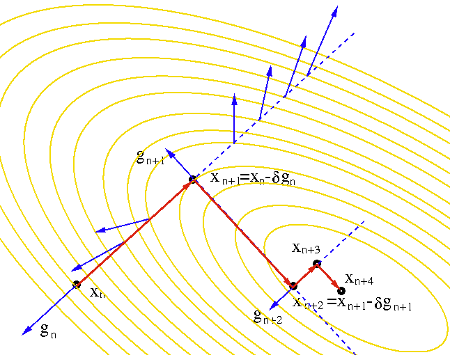
The reason why ${\bf g}_{n+1}\perp{\bf g}_n$ can also be explained geometrically. As shown in the figure the gradient vectors at various points along the direction of $-{\bf g}_n$ are shown by the blue arrows, and their projections onto the direction represent the slopes of the function $f(\delta_n)=f({\bf x}_n-\delta_n{\bf g}_n)$. Obviously at ${\bf x}_{n+1}$ where $f(\delta_n)$ reaches its minimum, its slope is zero. In other words, the projection of the gradient ${\bf g}_{n+1}$ onto the direction of $-{\bf g}_n$ is zero, i.e., ${\bf g}_{n+1}\perp{\bf g}_n$ or ${\bf g}_{n+1}^T{\bf g}_n=0$.

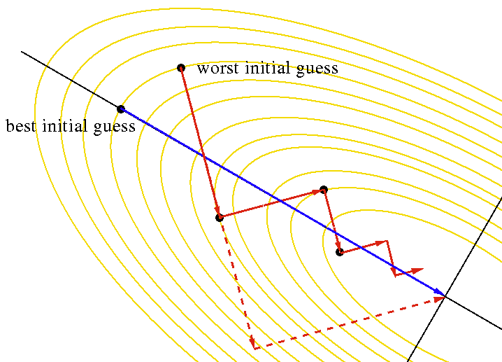
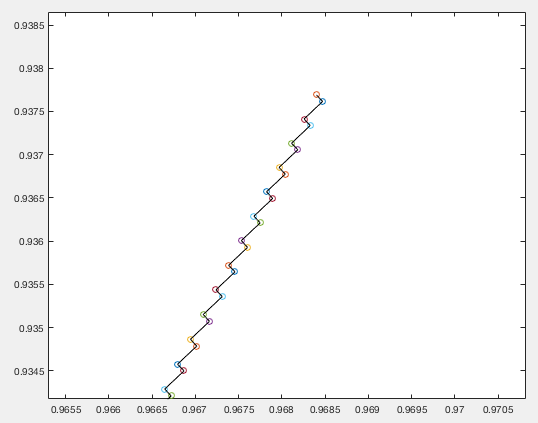
The gradient descent method gradually approaches a solution ${\bf x}$ of an N-D minimization problem by moving from the initial guess ${\bf x}_0$ along a zigzag path composed of a set of segments with any two consecutive segments perpendicular to each other. The number of steps depends greatly on the initial guess. As illustrated in the example below in an N=2 dimensional case, the best possible case is that the solution happens to be on the gradient direction of the initial guess, which could be reached in a single step, while the worst possible case is that the gradient direction of the initial guess happens to be 45 degrees off from the gradient direction of the optimal case, and it takes many zigzag steps to go around the optimal path to reach the solution. Many of the steps are in the same direction as some of the previous steps.

To improve the performance of the gradient descent method we can include in the iteration a momentum term representing the search direction previously traversed:

$${\bf x}_{n+1}={\bf x}_n-\delta_n{\bf g}_n+\alpha_n({\bf x}_n-{\bf x}_{n-1})$$ (77)

Now two consecutive search directions are no longer perpendicular to each other and the resulting search path is smoother than the zigzag path without the momentum term. The parameter $\alpha_m$ controls how much momentum is to be added.

Obviously it is most desirable not to repeat any of the previous directions traveled so that the solution can be reached in N steps, each in a unique direction in the N-D space. In other words, the subsequent steps are independent of each other, never interfering with the results achieved in the previous steps. Such a method will be discussed in the next section.

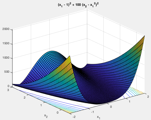
Example:

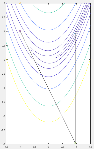
The Rosenbrock function

$$f(x,y)=(a-x)^2+b(y-x^2)^2\;\;\;\;\;\;\;\; \mbox{typically $a=1,\;b=100$}$$

is a two-variable non-convex function with a global minimum $f(1,\;1)=0$ at the point $(1,\;1)$, which is inside a long parabolic shaped valley as shown in the figure below. As the slope along the valley is very shallow, it is difficult for an algorithm to converge quickly to the minimum. For this reason, the Rosenbrock function is often used to test various minimization algorithms.

The figure below shows the search path of the gradient descent method based on the optimal step size given in Eq. (64). We see that the search path is composed a long sequence of 90 degree turns between consecutive segments.

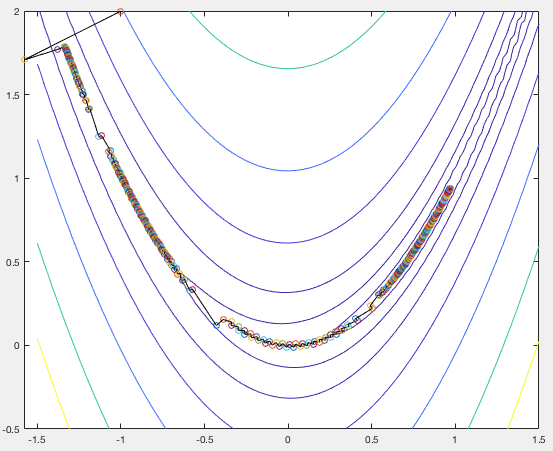
When the Newton's method is applied to this minimization problem, it takes only four iterations for the algorithm to converge to the minimum, as shown in the figure below: