Conjugate gradient method

The gradient descent method can be used to solve the minimization problem when the Hessian matrix of the objective function is not available. However, this method may be inefficient if it gets into a zigzag search pattern and repeat the same search directions many times. This problem can be avoided in the conjugate gradient (CG) method. If the objective function is quadratic, the CG method converges to the solution in $N$ iterations without repeating any of the directions previously traversed. If the objective function is not quadratic, the CG method can still significantly improve the performance in comparison to the gradient descent method.

Again consider the approximation of the function $f({\bf x})$ to be minimized by the first three terms of its Taylor series:

$$f({\bf x})=f({\bf x}_0+\delta{\bf x}) \approx f({\bf x}_0)+{\bf g}_0^T\delta{\bf x} +\frac{1}{2}\delta{\bf x}^T{\bf H}_0\delta{\bf x}$$ (128)

If the Hessian matrix is positive definite, then $f({\bf x})$ has a minimum. If function $f({\bf x})$ is quadratic, the approximation above becomes exact and the function can be written as

$$f({\bf x})=\frac{1}{2}{\bf x}^T{\bf A}{\bf x}-{\bf b}^T{\bf x}+c$$ (129)

where ${\bf A}={\bf H}$ is the symmetric Hessian matrix, and its gradient and Hessian can be written as the following respectively:

$${\bf g}({\bf x})=\frac{d}{d{\bf x}}f({\bf x}) =\frac{d}{d{\bf x}}... ...1}{2}{\bf x}^T{\bf A}{\bf x} -{\bf b}^T{\bf x}+c\right) ={\bf A}{\bf x}-{\bf b}$$ (130)

and

$${\bf H}({\bf x})=\frac{d^2}{d{\bf x}^2}f({\bf x})=\frac{d}{d{\bf x}}{\bf g} =\frac{d}{d{\bf x}}({\bf Ax}-{\bf b})={\bf A}$$ (131)

Solving ${\bf g}({\bf x})={\bf A}{\bf x}-{\bf b}={\bf0}$, we get the solution ${\bf x}^*={\bf A}^{-1}{\bf b}$, at which the function is minimized to

$$f({\bf x}^*)=\frac{1}{2}({\bf A}^{-1}{\bf b})^T{\bf A}({\bf A}^{-... ...}) -{\bf b}^T({\bf A}^{-1}{\bf b})+c=-\frac{1}{2}{\bf b}^T{\bf A}^{-1}{\bf b}+c$$ (132)

At the solution ${\bf x}^*$ that minimizes $f({\bf x})$, its gradient is

$${\bf g}({\bf x}^*)={\bf A}{\bf x}^*-{\bf b}={\bf0}$$ (133)

We also see that the minimization of the quadratic function $f({\bf x})$ is equivalent to solving a linear equation ${\bf A}{\bf x}={\bf b}$ with a symmetric positive definite coefficient matrix ${\bf A}$. The CG method considered here can therefore be used for solving both problems.

Conjugate basis vectors

We first review the concept of conjugate vectors, which is of essential importance in the CG method. Two vectors ${\bf u}$ and ${\bf v}$ are mutually conjugate (or A-orthogonal or A-conjugate) to each other with respect to a symmetric matrix ${\bf A}={\bf A}^T$, if they satisfy:

$${\bf u}^T{\bf A}{\bf v}=({\bf A}{\bf v})^T{\bf u} ={\bf v}^T{\bf A}{\bf u}=0$$ (134)

Specially, if ${\bf A}={\bf I}$, the two conjugate vectors become orthogonal to each other, i.e., ${\bf v}^T{\bf u}=0$.

Similar to a set of $N$ orthogonal vectors that can be used as the basis spanning an N-D space, a set of $N$ mutually conjugate vectors $\{{\bf d}_0,\cdots,{\bf d}_{N-1}\}$ satisfying ${\bf d}_i^T{\bf A}{\bf d}_j=0$ ($i\ne j$) can also be used as a basis to span the N-D space. Any vector in the space can be expressed as a linear combination of these basis vectors.

Also we note that any set of $N$ independent vectors can be converted by the Gram-Schmidt process to a set of $N$ basis vectors that are either orthogonal or A-orthogonal.

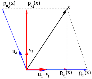
Example:

Given two independent basis vectors of the 2-D space, and a positive-definite matrix:

$${\bf v}_1=\left[\begin{array}{r}1\\ 0\end{array}\right],\;\;\;\;\... ...y}\right],\;\;\;\;\; {\bf A}=\left[\begin{array}{rr}3&1\\ 1&2\end{array}\right]$$

we can construct two A-orthogonal basis vectors by the Gram-Schmidt method:

$${\bf u}_1={\bf v}_1=\left[\begin{array}{r}1\\ 0\end{array}\right]... ...1^T{\bf A}{\bf u}_1}{\bf u}_1 =\left[\begin{array}{c}-1/3\\ 1\end{array}\right]$$

The projections of a vector ${\bf x}=[2,\;3]^T$ onto ${\bf v}_1$ and ${\bf v}_2$ are:

$${\bf p}_{{\bf v}_1}({\bf x})=\frac{{\bf v}_1^T{\bf x}}{{\bf v}_1^... ...array}{c}0\\ 1\end{array}\right] =\left[\begin{array}{c}0\\ 3\end{array}\right]$$

The A-projections of the same vector ${\bf x}$ onto ${\bf u}_1$ and ${\bf u}_2$ are:

$${\bf p}_{{\bf u}_1}({\bf x})=\frac{{\bf u}_1^T{\bf A}{\bf x}} {{\... ...y}{c}-1/3\\ 1\end{array}\right] =\left[\begin{array}{c}-1\\ 3\end{array}\right]$$

The original vector ${\bf x}$ can be represented in either of the two bases:

$${\bf x}=\left[\begin{array}{c}2\\ 3\end{array}\right] = 2\left[\begin{array}{c}1\\ 0\end{array}\right] +3\left[\begin{arr... ...{\bf v}_1+3{\bf v}_2 ={\bf p}_{{\bf v}_1}({\bf x})+{\bf p}_{{\bf v}_2}({\bf x})$$

$$= 3\left[\begin{array}{c}1\\ 0\end{array}\right] +3\left[\begin{arr... ...{\bf u}_1+3{\bf u}_2 ={\bf p}_{{\bf u}_1}({\bf x})+{\bf p}_{{\bf u}_2}({\bf x})$$

Search along a conjugate basis

Similar to the gradient descent method, which iteratively improves the estimated solution by following a sequence of orthogonal search directions $\{ {\bf d}_0,\cdots,{\bf d}_n,\cdots \}$ with ${\bf d}_n=-{\bf g}_n$ satisfying ${\bf g}_n^T{\bf g}_{n+1}=0$, the CG method also follows a sequence of search directions $\{{\bf d}_0,\cdots,{\bf d}_{N-1}\}$ A-orthogonal to each other, i.e., ${\bf d}_i^T{\bf Ad}_j=0\;(i\ne j)$:

$${\bf x}_{n+1}={\bf x}_n+\delta_n{\bf d}_n =\cdots ={\bf x}_0+\sum_{i=0}^n \delta_i{\bf d}_i$$ (135)

We define the error at the nth step as ${\bf e}_n={\bf x}_n-{\bf x}^*$. Then subtracting ${\bf x}^*$ from both sides, we get the iteration in terms of the errors:

$${\bf e}_{n+1}={\bf e}_n+\delta_n{\bf d}_n =\cdots={\bf e}_0+\sum_{i=0}^n \delta_i{\bf d}_i$$ (136)

Due to ${\bf g}={\bf Ax}-{\bf b}$ in Eq. (133), we can find the gradient at the nth step ${\bf x}_n$ as

$${\bf g}_n ={\bf A}{\bf x}_n-{\bf b} ={\bf A}({\bf x}^*+{\bf e}_n)-{\bf b} ={\bf A}{\bf x}^*-{\bf b}+{\bf A}{\bf e}_n={\bf A}{\bf e}_n$$ (137)

As the gradient at the solution is zero ${\bf g}({\bf x}^*)={\bf0}$, we can consider the gradient ${\bf g}_n$ at ${\bf x}_n$ as the residual of the nth iteration, and $\varepsilon=\vert\vert{\bf g}_n\vert\vert^2$ an error measurement representing how close ${\bf x}_n$ is to the true solution ${\bf x}^*$.

The optimal step size given in Eq. (60) can now be written as

$$\delta_i = -\frac{{\bf d}_i^T{\bf g}_i}{{\bf d}_i^T{\bf A}{\bf d}_i} =-\frac... ...bf e}_0+\sum_{j=0}^{i-1}\delta_j{\bf d}_n\right)} {{\bf d}^T_i{\bf A}{\bf d}_i}$$

$$= -\frac{ {\bf d}^T_i{\bf A}{\bf e}_0+\sum_{j=0}^{n-1}\delta_j{\bf ... ...}{\bf d}_i} =-\frac{ {\bf d}^T_i{\bf A}{\bf e}_0}{ {\bf d}^T_i{\bf A}{\bf d}_i}$$ (138)

The last equality is due to the fact that ${\bf d}_i$ and ${\bf d}_j$ are A-orthogonal, ${\bf d}^T_i{\bf A}{\bf d}_j=0$. Substituting this into Eq. (136) we get

$${\bf e}_{n+1}={\bf e}_n+\delta_n{\bf d}_n ={\bf e}_n-\left(\frac{{\bf d}_n^T{\bf A}{\bf e}_0} {{\bf d}_n^T{\bf A}{\bf d}_n}\right){\bf d}_n$$ (139)

On the other hand, we can represent the error ${\bf e}_0={\bf x}_0-{\bf x}^*$ associated with the initial guess ${\bf x}_0$ as a linear combination of the A-orthogonal search vectors $\{{\bf d}_0,\cdots,{\bf d}_{N-1}\}$ as $N$ basis vectors that span the N-D vector space:

$${\bf e}_0=\sum_{i=0}^{N-1} c_i{\bf d}_i =\sum_{i=0}^{N-1}{\bf p}_... ...ac{ {\bf d}^T_i{\bf A}{\bf e}_0} { {\bf d}^T_i{\bf A}{\bf d}_i}\right){\bf d}_i$$ (140)

where ${\bf p}_{{\bf d}_i}({\bf e}_0)$ is the A-projection of ${\bf e}_0$ onto the ith basis vector ${\bf d}_i$:

$${\bf p}_{{\bf d}_i}({\bf e}_0)=c_i{\bf d}_i =\left(\frac{ {\bf d}^T_i{\bf A}{\bf e}_0}{ {\bf d}^T_i{\bf A}{\bf d}_i}\right) {\bf d}_i$$ (141)

Note that the coefficient $c_i$ happens to be the negative optimal step size in Eq. (138):

$$c_i=\frac{{\bf d}^T_i{\bf A}{\bf e}_0}{{\bf d}^T_i{\bf A}{\bf d}_i}=-\delta_i$$ (142)

Now the expression of ${\bf e}_{n+1}$ in Eq. (136) can be written as

$${\bf e}_{n+1}={\bf e}_0+\sum_{i=0}^n\delta_i{\bf d}_i =\sum_{i=0}... ...sum_{i=n+1}^{N-1}c_i{\bf d}_i =\sum_{i=n+1}^{N-1}{\bf p}_{{\bf d}_i}({\bf e}_0)$$ (143)

We see that in each iteration, the number of terms in the summation for ${\bf e}_0$ is reduced by one, i.e., the nth component ${\bf p}_{{\bf d}_n}({\bf e}_0)$ of ${\bf e}_0$ along the direction of ${\bf d}_n$ is completely eliminated. After $N$ such iterations, the error is reduced from ${\bf e}_0$ to ${\bf e}_N={\bf0}$, and the true solution is obtained ${\bf x}_N={\bf x}^*+{\bf e}_N={\bf x}^*$.

Pre-multiplying ${\bf d}_k^T{\bf A}\;(k\le n)$ on both sides of the equation above, we get

$${\bf d}_k^T{\bf A}{\bf e}_{n+1} =\sum_{i=n+1}^{N-1}c_i{\bf d}_k^T{\bf A}{\bf d}_j=0$$ (144)

We see that after $n+1$ iterations the remaining error ${\bf e}_{n+1}$ is A-orthogonal to all previous directions ${\bf d}_0,\cdots,{\bf d}_n$.

Due to Eq. (137), the equation above can also be written as

$${\bf d}_k^T{\bf A}{\bf e}_{n+1}={\bf d}_k^T{\bf g}_{n+1}=0$$ (145)

i.e., the gradient ${\bf g}_{n+1}$ is orthogonal to all previous search directions.

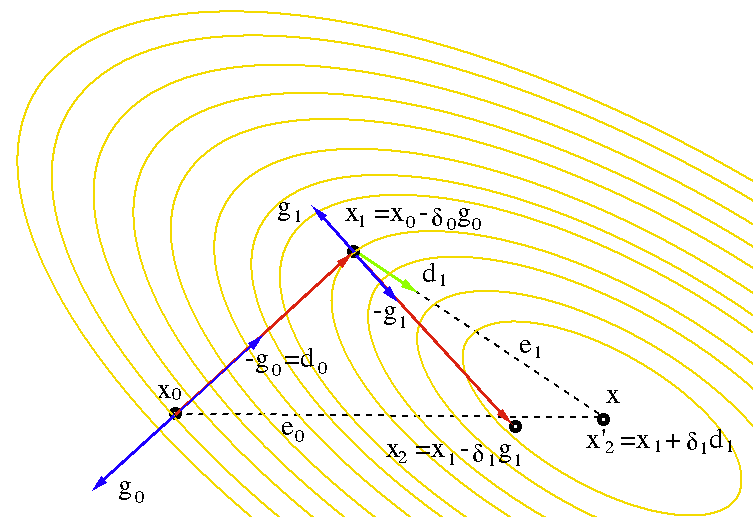
In the figure below, the conjugate gradient method is compared with the gradient descent method for the case of $N=2$. We see that the first search direction is the same $-{\bf g}_0$ for both methods. However, the next search direction ${\bf d}_1$ is A-orthogonal to ${\bf d}_0$, same as the next error ${\bf e}_1$, different from the search direction $-{\bf g}_1$ in gradient descent method. The conjugate gradient method finds the solution ${\bf x}$ in $N=2$ steps, while the gradient descent method has to go through many more steps all orthogonal to each other before it finds the solution.

.

Find the A-orthogonal basis

The $N$ A-orthogonal search directions $\{{\bf d}_0,\cdots,{\bf d}_{N-1}\}$ can be constructed based on any set of $N$ independent vectors $\{{\bf v}_0,\cdots,{\bf v}_{N-1}\}$ by the Gram-Schmidt process:

$${\bf d}_n={\bf v}_n-\sum_{j=0}^{n-1} {\bf p}_{{\bf d}_j}({\bf v}_... ...f A}{\bf d}_m}\right) {\bf d}_m ={\bf v}_n-\sum_{m=0}^{n-1} \beta_{nm}{\bf d}_m$$ (146)

where $\beta_{nm}={\bf d}^T_m{\bf A}{\bf v}_n/({\bf d}^T_m{\bf A}{\bf d}_m)$ and $\beta_{nm}{\bf d}_m$ is the A-projection of ${\bf v}_n$ onto each of the previous direction ${\bf d}_m$.

We will gain some significant computational advantage if we choose to use ${\bf v}_n=-{\bf g}_n$. Now the Gram-Schmidt process above becomes:

$${\bf d}_n =-{\bf g}_n-\sum_{m=0}^{n-1} \beta_{nm}{\bf d}_m,$$ (147)

where

$$\beta_{nm}=\frac{{\bf d}_m^T{\bf A}{\bf v}_n}{{\bf d}^T_m{\bf A}{... ...rac{{\bf d}_m^T{\bf A}{\bf g}_n}{{\bf d}^T_m{\bf A}{\bf d}_m} \;\;\;\;\;\;(m<n)$$ (148)

The equation above indicates that ${\bf g}_n$ can be written as a linear combination of all previous search directions ${\bf d}_0,\cdots,{\bf d}_n$:

$${\bf g}_n=\sum_{i=0}^n \alpha_i{\bf d}_i$$ (149)

Pre-multiplying ${\bf g}_{n+1}^T$ on both sides, we get

$${\bf g}_{n+1}^T{\bf g}_k={\bf g}_{n+1}^T\left( \sum_{i=0}^k \alpha_i{\bf d}_i\right) =\sum_{i=0}^k \alpha_i\;{\bf g}_{n+1}^T{\bf d}_i=0$$ (150)

The last equality is due to ${\bf g}_{n+1}^T{\bf d}_k=0$ in Eq. (145). We see that ${\bf g}_{n+1}$ is also orthogonal to all previous gradients ${\bf g}_0,\cdots,{\bf g}_n$.

Pre-multiplying ${\bf g}_k^T (k\ge n)$ on both sides of Eq. (147), we get

$${\bf g}_k^T{\bf d}_n=-{\bf g}_k^T{\bf g}_n-\sum_{m=0}^{n-1} \beta... ...\begin{array}{cc}-\vert\vert{\bf g}_n\vert\vert^2&n=k\\ 0&n<k\end{array}\right.$$ (151)

Note that all terms in the summation are zero as ${\bf g}_k^T{\bf d}_m=0$ for all $m<n\le k$ (Eq. (145)). Substituting ${\bf g}_n^T{\bf d}_n=-\vert\vert{\bf g}_n\vert\vert^2$ into Eq. (138), we get

$$\delta_n=-\frac{{\bf g}_n^T{\bf d}_n}{{\bf d}_n^T{\bf A}{\bf d}_n} =\frac{\vert\vert{\bf g}_n\vert\vert^2}{{\bf d}_n^T{\bf A}{\bf d}_n}$$ (152)

Next we consider

$${\bf g}_{m+1}={\bf A}{\bf x}_{m+1}-{\bf b} ={\bf A}({\bf x}_m+\de... ...{\bf x}_m-{\bf b})+\delta_m{\bf A}{\bf d}_m ={\bf g}_m+\delta_m{\bf A}{\bf d}_m$$ (153)

Pre-multiplying ${\bf g}_n^T$ with $n>m$ on both sides we get

$${\bf g}_n^T{\bf g}_{m+1}={\bf g}_n^T{\bf g}_m+\delta_m{\bf g}_n^T{\bf A}{\bf d}_m =\delta_m{\bf g}_n^T{\bf A}{\bf d}_m$$ (154)

where ${\bf g}_n^T{\bf g}_m=0$ ($m\ne n$). Solving for ${\bf g}_n^T{\bf A}{\bf d}_m$ we get

$${\bf g}_n^T{\bf A}{\bf d}_m =\frac{1}{\delta_m} {\bf g}_n^T{\bf g... ... \vert\vert{\bf g}_n\vert\vert^2/\delta_{n-1}&m=n-1\\ 0&m<n-1\end{array}\right.$$ (155)

Substituting this into Eq. (148) we get

$$\beta_{nm}=-\frac{{\bf d}_m^T{\bf A}{\bf g}_n}{{\bf d}^T_m{\bf A}... ...ta_{n-1}{\bf d}_{n-1}^T{\bf A}{\bf d}_{n-1} &m=n-1 \\ 0&m<n-1\end{array}\right.$$ (156)

which is non-zero only when $m=n-1$, i.e., there is only one non-zero term in the summation of the Gram-Schmidt formula for ${\bf d}_n$. This is the reason why we choose ${\bf v}_n=-{\bf g}_n$. We can now drop the second subscript $m$ in $\beta_{nm}$, and Eq. (146) becomes:

$${\bf d}_n={\bf v}_n-\sum_{m=0}^{n-1} \beta_{nm}{\bf d}_m =-{\bf g}_n-\beta_n{\bf d}_{n-1}$$ (157)

Substituting the step size $\delta_{n-1}=\vert\vert{\bf g}_{n-1}\vert\vert^2/{\bf d}_{n-1}^T{\bf A}{\bf d}_{n-1}$ (Eq. (152)) into the above expression for $\beta_{nm}=\beta_m$, we get

$$\beta_n=-\frac{\vert\vert{\bf g}_n\vert\vert^2}{\vert\vert{\bf g}_{n-1}\vert\vert^2}$$ (158)

We note that matrix ${\bf A}$ no longer appears in the expression.

The CG algorithm

Summarizing the above, we finally get the conjugate gradient algorithm in the following steps:

1. Set $n=0$ and initialize the search direction (same as gradient descent):

   $${\bf d}_0=-{\bf g}_0$$ (159)

2. Terminate if the error $\varepsilon=\vert\vert{\bf g}_n\vert\vert^2$ is smaller than a preset threshold. Otherwise, continue with the following:
3. Find optimal step size (Eq. (152)) and step forward

   $$\delta_n=\frac{\vert\vert{\bf g}_n\vert\vert^2}{{\bf d}_n^T{\bf A}{\bf d}_n}, \;\;\;\;\;\;\;\; {\bf x}_{n+1}={\bf x}_n+\delta_n{\bf d}_n$$ (160)

4. Update gradient:

   $${\bf g}_{n+1}=\frac{d}{d{\bf x}}f({\bf x}_{n+1})$$ (161)

5. Find coefficient for the Gram-Schmidt process (Eq. (158):

   $$\beta_{n+1}=-\frac{\vert\vert{\bf g}_{n+1}\vert\vert^2}{\vert\vert{\bf g}_n\vert\vert^2}$$ (162)

6. Update search direction (Eq. (157)):

   $${\bf d}_{n+1}=-{\bf g}_{n+1}-\beta_{n+1}{\bf d}_n$$ (163)

   Set $n=n+1$ and go back to step 2.

The algorithm above assumes the objective function $f({\bf x})$ to be quadratic with known ${\bf A}$. But when $f({\bf x})$ is not quadratic, ${\bf A}$ is no longer available, we can still approximate $f({\bf x})$ as a quadratic function by the first three terms in its Taylor series in the neighborhood of its minimum. Also, the we need to modify the algorithm so that it does not depend on ${\bf A}$. Specifically, the optimal step size $\delta_n$ calculated in step 3 above based on ${\bf A}$ can also be alternatively found by line minimization based on any suitable algorithms for 1-D optimization.

The Matlab code for the conjugate gradient algorithm is listed below:

function xn=myCG(o,tol)       % o is the objective function to minimize
    syms d;                   % variable for 1-D symbolic function f(d)
    x=symvar(o).';            % symbolic variables in objective function
    O=matlabFunction(o);      % the objective function
    G=jacobian(o).';          % symbolic gradient of o(x)
    G=matlabFunction(G);      % the gradient function
    xn=zeros(length(x),1);    % initial guess of x
    xc=num2cell(xn);
    e=O(xc{:});               % initial error
    gn=G(xc{:});              % gradient at xn
    dn=-gn;                   % use negative gradient as search direction
    n=0;
    while e>tol
        n=n+1;
        f=subs(o,x,xn+d*dn);          % convert n-D f(x) to 1-D f(d)
        delta=Opt1d(f);               % find delta that minimizes 1D function f(d)
        xn=xn+delta*dn;               % updata variable x
        xc=num2cell(xn);
        e=O(xc{:});                   % new error
        gn1=G(xc{:});                 % new gradient
        bt=-(gn1.'*gn1)/(gn.'*gn);    % find beta
        dn=-gn1-bt*dn;                % new search direction
        gn=gn1;                       % update gradient
        fprintf('%d\t(%.4f, %.4f, %.4f)\t%e\n',n,xn(1),xn(2),xn(3),e)
    end
end

Here is the function that uses Newton's method to find the optimal step size $\delta$ that minimizes the objective function as a 1-D function of $\delta$:

function x=Opt1d(f)         % f is 1-D symbolic function to minimize
    syms x;
    tol=10^(-3); 
    d1=diff(f);             % 1st order derivative
    d2=diff(d1);            % 2nd order derivative
    f=matlabFunction(f);
    d1=matlabFunction(d1);
    d2=matlabFunction(d2);
    x=0.0;                  % initial guess of delta
    if d2(x)<=0             % second order derivative needs to be greater than 0
        x=rand-0.5;
    end
    y=x+1;
    while abs(x-y) > tol    % minimization
        y=x;
        x=y-d1(y)/d2(y);    % Newton iteration
    end
end

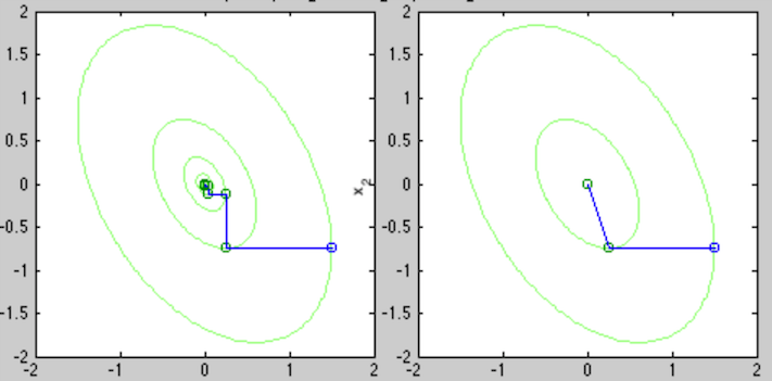
Example:

To compare the conjugate method and the gradient descent method, consider a very simple 2-D quadratic function

$$f(x,y)={\bf x}^T{\bf A}{\bf x} =[x_1,\,x_2]\left[\begin{array}{cc}3&1\\ 1&2\end{array}\right] \left[\begin{array}{c}x_1\\ x_2\end{array}\right]$$

The performance of the gradient descent method depends significantly on the initial guess. For the specific initial guess of ${\bf x}_0=[1.5,\;-0.75]^T$, the iteration gets into a zigzag pattern and the convergence is very slow, as shown below:

$$\begin{array}{c\vert c\vert c}\hline n & {\bf x}=[x_1,\,x_2] ... ... 13 & 0.000005, -0.000016 & 2.153408e-10 \\ \hline \end{array}$$

However, as expected, the conjugate gradient method takes exactly $N=2$ steps from any initial guess to reach at the solution:

$$\begin{array}{c\vert c\vert c}\hline n & {\bf x}=[x_1,\,x_2] ... ...\ 2 & 0.000000, -0.000000 & 1.155558e-33 \\ \hline \end{array}$$

For an $N=3$ example of $f({\bf x})={\bf x}^T{\bf A}{\bf x}$ with

$${\bf A}=\left[\begin{array}{ccc}5 & 3 & 1\\ 3 & 4 & 2\\ 1 & 2 & 3 \end{array}\right]$$

from an initial guess ${\bf x}_0=[1,\;2,\;3]^T$, it takes the gradient descent method 41 iterations to reach ${\bf x}_{41}=[3.5486e-06,\;-7.4471e-06,\;4.6180e-06]^T$ corresponding to $f({\bf x})=8.5429e-11$. From the same initial guess, it takes the conjugate gradient method only $N=3$ iterations to converge to the solution:

$$\begin{array}{c\vert c\vert c}\hline n & {\bf x}=[x_1,\,x_2,\... ...000000, 0.000000, 0.000000 & 3.949119e-31 \\ \hline \end{array}$$

For an $N=9$ example, it takes over 4000 iterations for the gradient descent method to converge with $\vert\vert{\bf e}\vert\vert\approx 10^{-10}$, but exactly 9 iterations for the CG method to converge with $\vert\vert{\bf e}\vert\vert\approx 10^{-16}$.

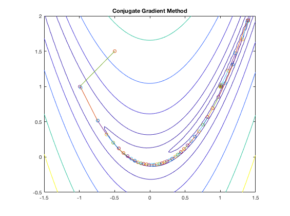
Example:

The figure below shows the search path of the conjugate gradient method applied to the minimization of the Rosenbrock function:

Example:

Solve the following $N=3$ non-linear equation system by the CG method:

$$\left\{\begin{array}{l} f_1(x_1,\,x_2,\,x_3)=3x_1-(x_2x_3)^2-3/2\... ...25\,x_2^2+2x_2-1\\ f_3(x_1,\,x_2,\,x_3)=exp(-x_1x_2)+20x_3+9\end{array}\right.$$

The solution is known to be $x_1=0.5,\;x_2=0,\;x_3=-0.5$.

This equation system can be represented in vector form as ${\bf f}({\bf x})={\bf0}$ and the objective function is $o({\bf x})={\bf f}^T({\bf x}){\bf f}({\bf x})$. The iteration of the CG method with an initial guess ${\bf x}_0={\bf0}$ is shown below:

$$\begin{array}{c\vert c\vert c}\hline n & {\bf x}=[x_1,\,x_2,\... ...& 0.5000, -0.0000, -0.5000 & 4.463926e-09 \\ \hline \end{array}$$

In comparison, the gradient descent method would need to take over 200 iterations (with much reduced complexity though) to reach this level of error.

Conjugate gradient method used for solving linear equation systems:

As discussed before, if ${\bf x}$ is the solution that minimizes the quadratic function $f({\bf x})={\bf x}^T{\bf A}{\bf x}/2-{\bf b}^T{\bf x}+c$, with ${\bf A}={\bf A}^T$ being symmetric and positive definite, it also satisfies $d\,f({\bf x})/d{\bf x}={\bf A}{\bf x}-{\bf b}={\bf0}$. In other words, the optimization problem is equivalent to the problem of solving the linear system ${\bf A}{\bf x}-{\bf b}={\bf0}$, both can be solved by the conjugate gradient method.

Now consider solving the linear system ${\bf A}{\bf x}={\bf b}$ with ${\bf A}={\bf A}^T$. Let ${\bf d}_i,\;(i=1,\cdots,N)$ be a set of $N$ A-orthogonal vectors satisfying ${\bf d}_i^T{\bf A}{\bf d}_j=0\;(i\ne j)$, which can be generated based on any $N$ independent vectors, such as the standard basis vectors, by the Gram-Smidth method. The solution ${\bf x}$ of the equation ${\bf A}{\bf x}={\bf b}$ can be represented by these $N$ vectors as

$${\bf x}=\sum_{i=1}^N c_i{\bf d}_i$$ (164)

Now we have

$${\bf b}={\bf A}{\bf x}={\bf A}\left[\sum_{i=1}^N c_i{\bf d}_i\right] =\sum_{i=1}^N c_i{\bf A}{\bf d}_i$$ (165)

Pre-multiplying ${\bf d}_j^T$ on both sides we get

$${\bf d}_j^T{\bf b}=\sum_{i=1}^N c_i{\bf d}_j^T{\bf A}{\bf d}_i=c_j{\bf d}_j^T{\bf A}{\bf d}_j$$ (166)

Solving for $c_j$ we get

$$c_j=\frac{{\bf d}_j^T{\bf b}}{{\bf d}_j^T{\bf A}{\bf d}_j}$$ (167)

Substituting this back into the expression for ${\bf x}$ we get the solution of the equation:

$${\bf x}=\sum_{i=1}^N c_i{\bf d}_i =\sum_{i=1}^N \left(\frac{{\bf d}_i^T{\bf b}}{{\bf d}_i^T{\bf A}{\bf d}_i}\right) {\bf d}_i$$ (168)

Also note that as ${\bf b}={\bf A}{\bf x}$, the ith term of the summation above is simply the A-projection of ${\bf x}$ onto the ith direction ${\bf d}_i$:

$${\bf p}_{{\bf d}_i}({\bf x}) =\left(\frac{{\bf d}_i^T{\bf A}{\bf x}}{{\bf d}_i^T{\bf A}{\bf d}_i}\right){\bf d}_i$$ (169)

One application of the conjugate gradient method is to solve the normal equation to find the least-square solution of an over-constrained equation system ${\bf A}{\bf x}={\bf b}$, where the coefficient matrix ${\bf A}$ is $M$ by $N$ with rank $R=N<M$. As discussed previously, the normal equation of this system is

$${\bf A}^T{\bf A}{\bf x}={\bf A}^T{\bf b}$$ (170)

Here ${\bf A}^T{\bf A}$ is an $N$ by $N$ symmetric, positive definite matrix. This normal equation can be solved by the conjugate gradient method.