Fixed point iteration

To answer the question why the iterative method for solving nonlinear equations works in some cases but fails in others, we need to understand the theory behind the method, the fixed point of a contraction function. If a single variable function $g(x)$ satisfies

$$\vert g(x_1)-g(x_2)\vert\le k \vert x_1-x_2\vert,\;\;\;\;\;k\ge 0$$ (36)

it is Lipschitz continuous, and $k$ is a Lipschitz constant. Specially, if $k=1$, then $g(x)$ is a non-expansive function, if $0\le k < 1$, then $g(x)$ is a contraction function or simply a contraction. These concepts can be generated to functions of multivariables ${\bf x}=[x_1,\cdots,x_N]^T\in \mathbb{R}^N$ (a point in an N-D metric space $V$):

$$g_n({\bf x})=g_n(x_1,\cdots,x_N),\;\;\;\;\;\;\;\;\; (n=1,\cdots,N)$$ (37)

which can also be expressed in vector form:

$${\bf g}({\bf x})=[g_1({\bf x}),\cdots,g_N({\bf x})]^T$$ (38)

Definition: In a metric space $V$ with certain distance $d({\bf x},\,{\bf y})$ defined between any two points ${\bf x},\,{\bf y}\in V$, a function ${\bf g}: V \rightarrow V$ is a contraction if

$$d({\bf g}({\bf x}),\,{\bf g}({\bf y})) \le k\,d({\bf x},\,{\bf y})$$ (39)

The smallest $k$ value that satisfies the above is called the (best) Lipschitz constant.

In the following, we will use the p-norm of the vector ${\bf x}-{\bf y}$ defined below as the distance measurement:

$$d( {\bf x},\,{\bf y})=\vert\vert{\bf x}-{\bf y}\vert\vert _p =\left(\sum_{n=1}^N (x_n-y_n)^p \right)^{1/p}$$ (40)

where $p\ge 1$, e.g., $p=1,\,2,\infty$. Also, for conveninece, we can drop $p$ so that $d({\bf x},\,{\bf y})=\vert\vert{\bf x}-{\bf y}\vert\vert$.

Intuitively, a contraction reduces the distance between points in the space, i.e., it brings them closer together. A function ${\bf g}({\bf x})$ may not be a contraction through out its entire domain, but it can be a contraction in the neighborhood of a certain point ${\bf x}^*\in V$, in which any ${\bf x}$ is sufficiently close to ${\bf x}^*$ so that

$$d({\bf g}({\bf x}),{\bf g}({\bf x}^*))\le k\,d({\bf x},{\bf x}^*), \;\;\;\;\;\;0\le k<1,\;\;\; d({\bf x},{\bf x}^*)<\epsilon>0$$ (41)

Definition: A fixed point ${\bf x}^*$ of a function ${\bf g}({\bf x})$ is a point in its domain that is mapped to itself:

$${\bf x}^*={\bf g}({\bf x}^*)$$ (42)

We immediately have

$${\bf g}({\bf g}({\bf x}^*))={\bf g}^2({\bf x}^*)={\bf x}^*, \cdot... ...f g}({\bf g}(\cdots {\bf g}({\bf x}^*)\cdots))) ={\bf g}^n({\bf x}^*)={\bf x}^*$$ (43)

A fixed point ${\bf x}^*$ is an attractive fixed point if any point $x$ in its neighborhood converges to ${\bf x}^*$, i.e., $\lim\limits_{n\rightarrow\infty}{\bf g}^n({\bf x})={\bf x}^*$.

Fixed Point Theorem : Let ${\bf g}({\bf x})$ be a contraction function satisfying

$$d( {\bf g}({\bf x})-{\bf g}({\bf y}) )\le k\; d({\bf x}-{\bf y}) \;\;\;\;\;\;(0\le k<1)$$ (44)

then there exists a unique fixed point ${\bf x}^*={\bf g}({\bf x}^*)$, which can be found by an iteration from an arbitrary initial point ${\bf x}_0$:

$$\lim\limits_{n\rightarrow\infty}{\bf x}_n =\lim\limits_{n\rightar... ...{n-2}) =\cdots =\lim\limits_{n\rightarrow\infty}{\bf g}^n({\bf x}_0) ={\bf x}^*$$ (45)

Proof

• We first prove constructively the existence of a fixed point. As ${\bf g}({\bf x})$ is a contraction, we have

  $$\vert\vert{\bf x}_{n+1}-{\bf x}_n\vert\vert=\vert\vert{\bf g}({\b... ... x}_{n-2}\vert\vert \le \cdots \le k^n \vert\vert {\bf x}_1-{\bf x}_0\vert\vert$$ (46)

  As $0\le k < 1$, we have $\lim\limits_{n\rightarrow\infty}\vert\vert{\bf x}_{n+1}-{\bf x}_n\vert\vert=0$. This is a Cauchy sequence that converges to some point $\lim\limits_{n\rightarrow\infty}{\bf x}_n={\bf x}^*$ also in the space. We further have

  $${\bf g}({\bf x}^*)={\bf g}(\lim\limits_{n\rightarrow\infty}{\bf x... ...fty}{\bf g}({\bf x}_n) =\lim\limits_{n\rightarrow\infty}{\bf x}_{n+1}={\bf x}^*$$ (47)

  i.e., the limit of the Cauchy sequence $\lim\limits_{n\rightarrow\infty}{\bf x}_n=x^*$ is a fixed point.

• We next prove the uniqueness of the fixed point. Let ${\bf x}^*_1$ and ${\bf x}^*_2$ be two fixed points of ${\bf g}({\bf x})$, then we have

  $$\vert\vert{\bf g}({\bf x}^*_1)-{\bf g}({\bf x}^*_2)\vert\vert\le ... ...^*_2\vert\vert =k \vert\vert{\bf g}({\bf x}^*_1)-{\bf g}({\bf x}^*_2)\vert\vert$$ (48)

  For any $k\ne 0$, the above holds only if $\vert\vert{\bf x}^*_1-{\bf x}^*_2\vert\vert=\vert\vert{\bf g}({\bf x}^*_1)-f({\bf x}^*_2)\vert\vert=0$, i.e., ${\bf x}^*_1={\bf x}^*_2$ is the unique fixed point.

QED

Theorem: Let ${\bf x}^*={\bf g}({\bf x}^*)$ be a fixed point of a differentiable function ${\bf g}({\bf x})$, i.e, $\partial g_i/\partial x_j$ exists for any $1\le i,j\le N$. If the norm of the Jacobian matrix is smaller than 1, $\vert\vert{\bf J}_{\bf g}({\bf x}^*)\vert\vert<1$, then ${\bf g}({\bf x})$ is a contraction at ${\bf x}^*$.

The Jacobian matrix of ${\bf g}({\bf x})$ is defined as

$${\bf g}'({\bf x})={\bf J}_{\bf g}({\bf x})=\left[\begin{array}{cc... ... g_N}{\partial x_1}&\cdots&\frac{\partial g_N}{\partial x_N} \end{array}\right]$$ (49)

Proof: Consider the Taylor expansion of the function ${\bf g}({\bf x})$ in the neighborhood of ${\bf x}^*$:

$${\bf g}({\bf x}) ={\bf g}({\bf x}^*)+{\bf g}'({\bf x}^*)({\bf x}-... ...({\bf x}^*)+{\bf J}_{\bf g}({\bf x}^*)({\bf x}-{\bf x}^*) +R({\bf x}-{\bf x}^*)$$ (50)

where $R({\bf x}-{\bf x}^*)$ is the remainder composed of second and higher order terms of ${\bf\delta}={\bf x}-{\bf x}^*$. Subtracting ${\bf g}({\bf x}^*)$ and taking any p-norm on both sides, we get

$$\vert\vert{\bf g}({\bf x})-{\bf g}({\bf x}^*)\vert\vert _p =\vert... ...{\bf J}_{\bf g}({\bf x}^*)({\bf x}-{\bf x}^*)+R({\bf x}-{\bf x}^*)\vert\vert _p$$ (51)

When ${\bf x}\rightarrow {\bf x}^*$, the second and higher order terms of ${\bf x-x}^*$ disappear and $R({\bf x}-{\bf x}^*)\rightarrow 0$, we have

$$\vert\vert{\bf g}({\bf x})-{\bf g}({\bf x}^*)\vert\vert _p =\vert... ...\bf g}({\bf x}^*) \vert\vert _p \cdot \vert\vert{\bf x}-{\bf x}^*\vert\vert _p,$$ (52)

The inequality is due to the Cauchy-Schwarz inequality. if $\vert\vert{\bf J}_{\bf g}({\bf x}^*)\vert\vert<1$, the function ${\bf g}({\bf x})$ is a contraction at ${\bf x}^*$.

QED

In particular, for a single-variable function in an $N=1$ dimensional space, we have

$$g(x)-g(x^*)=g'(x^*)(x-x^*)+\frac{1}{2}g''(x^*)(x-x^*)^2+R(x-x^*)$$ (53)

and

$$\vert g(x)-g(x^*)\vert\le\vert g'(x^*)(x-x^*)\vert\le\vert g'(x^*)\vert\;\vert(x-x^*)\vert$$ (54)

If $\vert g'(x)\vert<1$, then $g(x)$ is a contraction at $x^*$.

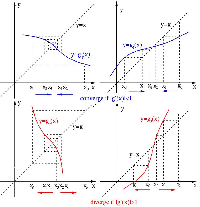
Now we understand why in the examples of the previous section the iteration leads to convergence in some cases but divergence in other cases: if $\vert g'(x)\vert<1$, the iteration will converge to the root $x^*$ of $f(x)=0$, but if $\vert g'(x)\vert>1$, it never will never converge.

The iterative process $x_{n+1}=g(x_n)$ for finding the fixed point of a single-variable function $g(x)$ can be shown graphically as the intersections of the function $y=g(x)$ and the identity function $y=x$, as shown below. The iteration converges in the first two cases as $\vert g'(x)\vert<1$, but it diverges in the last two cases as $\vert g'(x)\vert>1$.

We next find the order of convergence of the fixed point iteration. Consider

$$\lim\limits_{n\rightarrow\infty}\frac{\vert e_{n+1}\vert}{\vert e... ...y}\frac{\vert g(x_n)-g(x^*)\vert}{\vert x_n-x^*\vert} =\vert g'(x^*)\vert=\mu<1$$ (55)

We see that in general the fixed point iteration converges linearly. However, if the iteration function $g(x)$ has zero derivative at the fixed point $g'(x^*)=0$, we have

$$g(x)-g(x^*)=g'(x^*)(x-x^*)+\frac{1}{2}g''(x^*)(x-x^*)^2+R(x-x^*) =\frac{1}{2}g''(x^*)(x-x^*)^2+R(x-x^*)$$ (56)

and the iteration converges quadratically:

$$\lim\limits_{n\rightarrow\infty}\frac{\vert e_{n+1}\vert}{\vert e... ...vert g(x_n)-g(x^*)\vert}{\vert x_n-x^*\vert^2} =\frac{1}{2}\vert g''(x^*)\vert=$$ (57)

Moreover, if $g''(x^*)=0$, then the iteration converges cubically.

Consider a specific iteration function in the form of $g(x)=x-f(x)\phi(x)$, which is equivalent to $f(x)=0$, as if $x^*$ is the root of $f(x)$ satisfying $f(x^*)=0$, it also satisfies $g(x^*)=x^*$, which is indeed a fixed point of $g(x)$. The derivative of this function is

$$g'(x)=(x-f(x)\phi(x))'=1-f'(x)\phi(x)-f(x)\phi'(x) =1-f'(x)\phi(x)$$ (58)

If $f'(x)\ne 0$, then we can define $\phi(x)=1/f'(x)$ so that then $g'(x)=1-f'(x)/f'(x)=0$, then the convergence becomes quadratic. This is actually the Newton-Raphson method, to be discussed later.

Example 1

Find the solution of the following equation:

$$f(x)=x^3-x-2=0$$

This equation can converted into an equivalent form of $g(x)=x$ in two different ways:

$$g_1(x)=x=\sqrt[3]{x+2},\;\;\;\;\;\;\; \;\;\;\;\;\;g_2(x)=x=x^3-2$$

In the figure below, the two functions $g_1(x)$ (left) and $g_2(x)$ (right) together with $f(x)$ and the identity function are plotted:

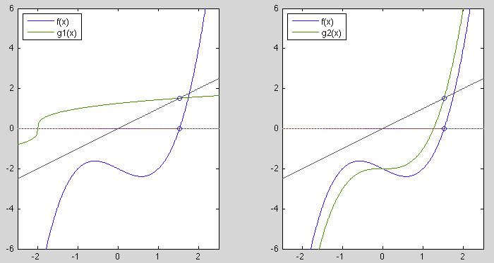
The iteration based on $g_1(x)$ converges to the solution $x^*=1.5214$ for any initial guess $-\infty<x_0<\infty$, as $g_1(x)$ is a contraction. However, the iteration based on $g_2(x)$ does not converge to $x^*$ as it is not a contraction in the neighborhood of $x^*$. In fact, the iteration will diverge towards either $-\infty$ if $x_0<x^*$ or $\infty$ if $x_0>x^*$.

Example 2

To solve the following equation

$$f(x)=x^3-3x+1=0$$

we first convert it into the form of $g(x)=x$ in two different ways:

$$g_1(x)=x=\sqrt[3]{3x-1},\;\;\;\;\;\;g_2(x)=x=\frac{1}{3}(x^3-1)$$

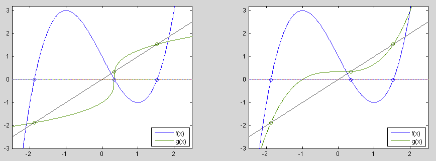
As can be seen in the plots, this equation has three solutions,

$$x_1=-1.8794,\;\;\;\;\;x_2=0.3473,\;\;\;\;\;\;x_3=1.5321$$

of which $x_1$ and $x_3$ can be obtained by the iteration based on $g_1(x)$ and $x_2$ can be obtained by the iteration based on $g_2(x)$. But neither of them can find all three roots.

• As shown in the plot on the left, $\vert g'_1(x)\vert<1$ for all $-\infty<x<\infty$ except in the neighborhood of $x_2=0.3473$, i.e., $g_1(x)$ is a contraction mapping everywhere except around $x_2$. Therefore the iteration starting from any initial guess $x_0$ will converge to either $x_1=-1.8749$ if $x_0<x_2$, or $x_3=1.5321$ if $x_0>x_2$.

  $$x_{n+1}=g_1(x_n)\stackrel{{n\rightarrow\infty}}{\Longrightarrow} ... ...n{array}{ll} x_1=-1.8749 & x_0<x_2 \\ x_3= 1.5321 & x_0>x_2 \end{array}\right.$$

  However, as $g_1(x)$ is not a contraction mapping around $x=x_2$, the iteration will never converge to $x_2$.
• As shown in the plot on the right, $\vert g'_2(x)\vert>1$ for all $-\infty<x<\infty$ except in the neighborhood of $x_2$, i.e., $g_2(x)$ is not a contraction mapping around either $x_1$ or $x_3$. Therefore the iteration based on $g_2(x)$ will not converge to either $x_1$ or $x_3$, but it may converge to $x_2$, if the initial guess $x_0$ is in the range $x_1<x_0<x_3$. However, if $x_0$ is outside this range the iteration will diverge toward either $-\infty$ if $x_0 < x_1$ of $\infty$ if $x_0>x_3$.

  $$x_{n+1}=g_2(x_n)\stackrel{{n\rightarrow\infty}}{\Longrightarrow} ... ...ty & x_0<x_1 \\ x_2=0.3473 & x_1<x_0<x_3 \\ \infty & x_0>x_3 \end{array}\right.$$

$$\begin{array}{r\vert c\vert c}\hline n & x_n & f(x_n) \\ \hli... ...line 12 & -1.8793853e+00 & -1.1116151e-06 \\ \hline \end{array}$$

Example 3

$$f(x)=\sin(x)-x^3=0$$

This equation can be converted into the form $g(x)=x$ in different ways:

• $$g_0(x)=x=\sqrt[3]{\sin(x)},\;\;\;\;g'_0(x)=\frac{\cos(x)}{3\,\sin(x)^{2/3}}$$

  $$\begin{array}{r\vert c\vert c}\hline n & x_n & f(x_n) \\ \hli... ... \\ \hline 8 & 9.286277e-01 & -2.7144e-06 \\ \hline \end{array}$$

• $$g_1(x)=x=\sin(x)/x^2,\;\;\;\;g'_1(x)=\frac{\cos(x)}{x^2}-\frac{2\,\sin(x)}{x^3}$$

• $$g_2(x)=x+\sin(x)-x^3,\;\;\;\;g'_2(x)=\cos(x)-3\,x^2+1$$

• $$g_3(x)=x-\frac{\sin(x)-x^3}{\cos(x)-3x^2},\;\;\;\; g'_3(x)=-\frac{(6x+\sin(x)) (\sin(x)-x^3)}{(\cos(x)-3x^2)^2}$$

$$\begin{array}{r\vert c\vert c}\hline n & x_n & f(x_n) \\ \hli... ... \\ \hline 6 & 9.286263e-01 & -8.9029e-11 \\ \hline \end{array}$$

Example 4

$$f(x)=e^x-\frac{1}{x}$$

• $$g_0(x)=x=e^{-x}, \;\;\;\;g'_0(x)=e^{-x}$$

  The iteration from any initial guess $x_0>0$ will converge to $x^*=g_1(x^*)=0.56714$.

• $$g_1(x)=x=-\log(x), \;\;\;\;g'_1(x)=1/x$$

  Around $x=x^*=0.56714$, $g'_1(x)=1/x>1$, the iteration does not converge.

• $$g_2(x)=x-\frac{e^x-1/x}{e^x+1/x^2}, \;\;\;\; g'_2(x)=\frac{(e^x-1/x)(e^x-2/x^3)}{(e^x+1/x^2)^2}$$

Example 5

Consider a 3-variable linear vector function ${\bf f}({\bf x})$ of arguments ${\bf x}=[x,\;y,\;z]^T$:

$${\bf f}({\bf x})={\bf0},\;\;\;\;\;\;\;\;\;\; \left\{ \begin{array... ...\\ f_2({\bf x})=2x+7y+3z-25=0\\ f_3({\bf x})=x+3y+5z-22=0 \end{array} \right.$$

from which the g-function can be obtained:

$${\bf g}({\bf x})={\bf x},\;\;\;\;\;\;\;\;\;\; \left\{ \begin{arra... ...g_2({\bf x})=y=-(2x+3z-25)/7\\ g_3({\bf x})=z=-(x+3y-22)/5 \end{array} \right.$$

The Jacobian ${\bf g}({\bf x})$ of this linear system is a constant matrix

$${\bf J}_g=\left[\begin{array}{rrr} 0 & -1/2 & -1/3\\ -2/7 & 0 & -3/7\\ -1/5 & -3/5 & 0 \end{array}\right]$$

with the induced p=2 norm (maximum singular value) $\vert\vert{\bf J}_g\vert\vert=0.851<1$. Consequently, the iteration ${\bf x}_{n+1}={\bf g}({\bf x}_n)$ converges from an initial guess ${\bf x}_0=[1,\,1,\,1]^T$ to the solution ${\bf x}=[1,\,2,\,3]^T$.

Alternatively, the g-function can also be obtained as

$${\bf g}'({\bf x})={\bf x},\;\;\;\;\;\;\;\;\;\; \left\{ \begin{arr... ...2({\bf x})=y=-(2x+3z-25)/7\\ g'_3({\bf x})=z=-(6x+3y-18)/2 \end{array} \right.$$

The Jacobian is

$${\bf J}_{g'}=\left[ \begin{array}{rrr} 0 & -3 & -5\\ -2/7 & 0 & -3/7\\ -3 & -3/2 & 0 \end{array}\right]$$

with the induced p=2 norm $\vert\vert{\bf J}_g\vert\vert=5.917>1$. The iteration does not converge.

Example 6

Consider a 3-variable nonlinear function ${\bf f}({\bf x})$ of arguments ${\bf x}=[x,\;y,\;z]^T$:

$${\bf f}({\bf x})={\bf0},\;\;\;\;\;\;\;\;\;\; \left\{ \begin{array... ...{\bf x})=xy^2-x-3y+yz+2=0\\ f_3({\bf x})=xz^2-3z+yz^2+xy=0 \end{array} \right.$$

The g-function can be obtained as

$${\bf g}({\bf x})={\bf x},\;\;\;\;\;\;\;\;\;\; \left\{ \begin{arra... ...bf x})=y=(xy^2-x+yz+2)/3\\ g_3({\bf x})=z=(xz^2+yz^2+xy)/3 \end{array} \right.$$

With ${\bf x}_0=[0,\;0,\;0]^T$ and after $n>170$ iterations ${\bf x}_{n+1}={\bf g}({\bf x}_n)$ converges to ${\bf x}_n=[1.098933,\;0.367621,\;0.144932]^T$, with error $\vert\vert{\bf f}({\bf x}_n)\vert\vert<10^{-7}$. However, the iteration may not converge from other possible initial guesses.

By Aitken's method, the iteration $x_{n+1}=g(x_n)$ can be accelerated based on two consecutive points $x_0$ and $x_1$, as shown in the figure below.

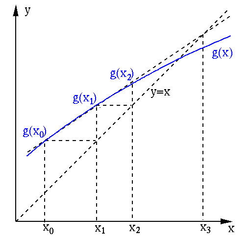
The secant line of $g(x)$ that goes through the two points $P_0=(x_0, g(x_0)=x_1)$ and $P_1=(x_1, g(x_1)=x_2)$ is represented by the equation in terms of its slope:

$$\frac{y-g(x_0)}{x-x_0}=\frac{g(x_1)-g(x_0)}{x_1-x_0}$$ (59)

Solving for $y$, we get

$$y=g(x_0)+(x-x_0)\frac{g(x_1)-g(x_0)}{x_1-x_0} =x_1+(x-x_0)\frac{x_2-x_1}{x_1-x_0}$$ (60)

To accelerate, instead of moving from $x_0$ to $x_1$, we move to the point $x$ at which this secant line intersects with the identity function $y=x$. We can therefore replace $y$ in the equation above by $x$ and solve the resulting equation

$$x=x_1+(x-x_0)\frac{x_2-x_1}{x_1-x_0}$$ (61)

to get

$$x=\frac{x_1(x_1-x_0)-x_0(x_2-x_1)}{(x_1-x_0)-(x_2-x_1)} =x_0-\frac{(x_1-x_0)^2}{x_2-2 x_1+x_0} =x_0-\frac{(\Delta x_0)^2}{\Delta^2 x_0}$$ (62)

where $\Delta x_0$ and $\Delta^2 x_0$ are respectively the first and second order differences defined below:

$$\Delta x_0=x_1-x_0,\;\;\;\;\;\Delta x_1=x_2-x_1$$ (63)

$$\Delta^2 x_0=\Delta x_1-\Delta x_0=(x_2-x_1)-(x_1-x_0)=x_2-2x_1+x_0$$ (64)

This result can then be converted into an iterative process

$$\left\{\begin{array}{l} x_{n+1}=g(x_n)\\ x_{n+2}=g(x_{n+1})\\ x_{n+3}=x_n-(x_{n+1}-x_n)^2/(x_{n+2}-2 x_{n+1}+x_n) \end{array}\right.$$ (65)

Given $x_n$, we skip $x_{n+1}=g(x_n)$ and $x_{n+2}=g(x_{n+1})$ but directly move to $x_{n+3}$ computed based on $x_{n+1}$ and $x_{n+2}$, thereby making a greater step towards the solution.

Example Solve $x^3-3x+1=0$. Construct $g(x)=(3x-1)^{1/3}$. It takes 18 iterations for the regular fixed point algorithm with initial guess $x_0=1$, to get $x_{18}=1.5320887$ that satisfies $\vert f(x_n)\vert<10^{-6}$, but it only three iterations for Aitken's method to converge to the same result:

$$\begin{array}{r\vert c\vert c}\hline n & x_n & f(x_n)\\ \hlin... ...6e-06\\ \hline 18& 1.532089 &-6.394874e-07\\ \hline \end{array}$$

$$\begin{array}{r\vert c\vert c}\hline n & x_n & f(x_n)\\ \hlin... ...e-03\\ \hline 3 & 1.5320889 & 3.421160e-08\\ \hline \end{array}$$