The Bisection and Secant methods

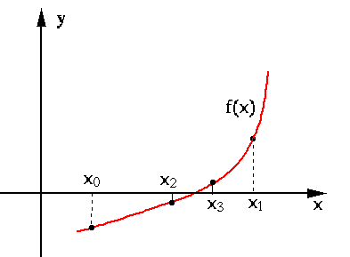
Here we consider a set of methods that find the solution $x^*$ of a single-variable nonlinear equation $f(x)=0$, by searching iteratively through a neighborhood of the domain, in which $x^*$ is known to be located.

The bisection search

This method requires two initial guesses $x_0 < x_1$ satisfying $f(x_0)f(x_1)<0$. As $f(x_0)$ and $f(x_1)$ are on opposite sides of the x-axis $y=0$, the solution $x^*$ at which $f(x^*)=0$ must reside somewhere in between of these two guesses, i.e., $x_0<x^*<x_1$.

Given such two end points $x_0$ and $x_1$, we find another point $x_2$ in between and use it to replace one of the end points at which the function value $f(x)$ has the same sign as that of $f(x_2)$. The new search interval is $a=x_2-x_0$ if $f(x_2)f(x_1)>0$, or $b=x_1-x_2$ if $f(x_0)f(x_2)>0$, either of which is smaller than the previous interval $a+b=x_1-x_0$. This process is then carried out iteratively until the solution is eventually approached, with a guaranteed convergence.

While any point between the two end points can be chosen for the next iteration, we want to avoid the worst possible case in which the solution always happens to be in the larger of the two sections $a$ and $b$. We can therefore choose the middle point between the two end points, i.e., $x_2=(x_0+x_1)/2$, so that $a=b=(x_1-x_0)/2$, i.e., the new search interval is always halved in each step of the iteration:

$$x_{n+1}=\frac{x_n+x_{n-1}}{2}$$ (11)

11

Here, without loss of generality, we have assumed $f(x_{n-1})f(x_{n+1})>0$ and $x_{n-1}$ is replaced by $x_{n+1}$.

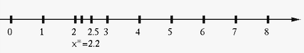
For example, we assume the root is located at $x^*=2.2$ between the two initial values are $x_0=0$ and $x_1=8$, then we get

$$\begin{array}{c\vert\vert c\vert c\vert c\vert c\vert c\vert ... ...& 0.2 & 0.8 & 0.3 & 0.05 & 0.075 & \cdots \\ \hline \end{array}$$ (12)

Note that the error $\vert e_n\vert=\vert x_n-x^*\vert$ does not necessarily always reduce monotonically. However, as in each iteration the search interval is always halved, the worst possible error is also halved:

$$\vert e_{n+1}\vert=\vert x_{n+1}-x^*\vert\le \frac{\vert x_n-x_{n-1}\vert}{2}=\frac{\vert x_0-x_1\vert}{2^n} \approx \frac{\vert e_n\vert}{2}$$ (13)

i.e., the convergence of the iteration is linear (of order $p=1$) and the rate of convergence is $1/2$:

$$\lim\limits_{n\rightarrow\infty}\frac{\vert e_{n+1}\vert}{\vert e... ...{n\rightarrow\infty}\frac{\vert e_{n+1}\vert}{\vert e_n\vert}\le\mu=\frac{1}{2}$$ (14)

14

Compared to other methods to be considered later, the bisection method converges rather slowly, but one of the advantages of the bisection method is that no derivative of the given function is needed. This means the given function $f(x)$ does not need to be differentiable.

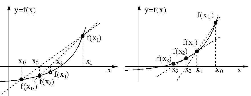
The Secant method

Same as in the bisection method, here again we assume there are two initial values $x_0$ and $x_1$ available, but they do not have to satisfy $f(x_0)f(x_1)<0$. Here the iteration is based on the zero-crossing of the secant line passing through the two points $f(x_0)$ and $f(x_1)$, instead of their middle point. The equation for the secant is:

$$\frac{y-f(x_0)}{x-x_0}=\frac{f(x_1)-f(x_0)}{x_1-x_0}$$ (15)

15

At the zero crossing, $y=0$ and the equation above can be solved for $x$, the position of the zero-crossing:

$$x=x_0-\frac{x_1-x_0}{f(x_1)-f(x_0)}f(x_0) =x_0-\frac{f(x_0)}{\hat{f}'(x_0)}$$ (16)

where $\hat{f}'(x_0)$ is the finite difference that approximates the derivative $f'(x_0)$:

$$\hat{f}'(x_0)=\frac{f(x_1)-f(x_0)}{x_1-x_0} =\frac{\Delta f(x_0)}{\Delta x_0}\;\; \stackrel{\Delta{x_0}\rightarrow 0}{\Longrightarrow} \;\;f'(x_0)$$ (17)

The new value $x$ obtained above, as a better estimate of the root than either $x_0$ or $x_1$, is used to replace one of them:

• If $f(x_0)f(x_1)<0$, then $x_i\;(i=0,\,1)$ satisfying $f(x_i)f(x)>0$ is replaced by $x_2=x$ (same as the bisection method);
• If $f(x_0)f(x_1)>0$, then $x_i\;(i=0,\,1)$ with greater $\vert f(x_i)\vert$ is replaced by $x_2=x$.

This process is then carried out iteratively to approach the root:

$$x_{n+1}=x_n-\frac{f(x_n)}{\hat{f}'(x_n)}$$ (18)

In case $f(x_n)=f(x_{n-1})$, the approximated derivative is zero $\hat{f}'(x_n)=0$, and $x_{n+1}$ cannot be found. In such a case, a root may exist between $x_n$ and $x_{n-1}$. Therefore the way to resolve this problem is to combine the bisection search with the secant method so that when $\hat{f}'=0$, the algorithm will switch to bisection search. This is Dekker's method:

$$x_{n+1}=\left\{\begin{array}{cl} x_n-f(x_n)/\hat{f}'(x_n) & \mbox{if}\;f(x_n)\ne f(x_{n-1})\\ (x_n+x_{n-1})/2 & \mbox{otherwise}\end{array}\right.$$ (19)

We now consider the order of convergence of the secant method. Let $x^*$ be the root at which $f(x^*)=0$. The error of $x_{n+1}$ is:

$$e_{n+1} = x_{n+1}-x^*=x_n-\frac{x_n-x_{n-1}}{f(x_n)-f(x_{n-1})}\,f(x_n)-x^*$$

$$= \frac{(x_{n-1}-x^*)f(x_n)-(x_n-x^*)f(x_{n-1}) }{f(x_n)-f(x_{n-1})} =\frac{e_{n-1}f(x_n)-e_nf(x_{n-1}) }{f(x_n)-f(x_{n-1})}$$ (20)

Consider the Taylor expansion of $f(x_n)$:

$$f(x_n)=f(x^*+e_n)=f(x^*)+f'(x^*)e_n+\frac{1}{2}f''(x^*)e_n^2+O(e_n^3) =f'(x^*)e_n+\frac{1}{2}f''(x^*)e_n^2+O(e_n^3)$$ (21)

(as $f(x^*)=0$) and similarly

$$f(x_{n-1})=f'(x^*)e_{n-1}+\frac{1}{2}f''(x^*)e_{n-1}^2+O(e_{n-1}^3)$$ (22)

Substituting these into the expression for $e_{n+1}$ above we get

$$e_{n+1} = \frac{e_{n-1}[f'(x^*)e_n+\frac{1}{2}f''(x^*)e_n^2+O(e_n^3)]-e_n[f... ...x^*)e_n^2+O(e_n^3)]-[f'(x^*)e_{n-1}+\frac{1}{2}f''(x^*)e_{n-1}^2+O(e_{n-1}^3)]}$$

$$= \frac{e_{n-1}e_nf''(x^*)(e_n-e_{n-1})/2+O(e_{n-1}^4)}{(e_n-e_{n-1})f'(x^*)+(e_n^2-e^2_{n+1})f''(x^*)/2+O(e_{n-1}^3)}$$

$$= \frac{e_{n-1}e_nf''(x^*)/2+O(e_{n-1}^3)}{f'(x^*)+(e_n+e_{n+1})f''(x^*)/2+O(e_{n-1}^2)}$$

$$= \frac{e_{n-1}e_nf''(x^*)/2+O(e_{n-1}^3)}{f'(x^*)+O(e_n)+O(e_{n-1}^2)}$$ (23)

When $n\rightarrow\infty$, the lowest order terms in both the numerator and denominator become the dominant terms as all other higher order terms approach to zero, and we have

$$e_{n+1}=\frac{e_{n-1}e_nf''(x^*)}{2f'(x^*)}=C\,e_ne_{n-1}$$ (24)

where we have defined a constant $C=f''(x^*)/2f'(x^*)$. To find the order of convergence, we need to find $p$ in

$$\vert e_{n+1}\vert\le\vert C\vert\;\vert e_{n-1}\vert\;\vert e_n\vert=\mu \vert e_n\vert^p$$ (25)

Solving this equation for $\vert e_n\vert$ we get

$$\vert e_n\vert=\left(\frac{\vert C\vert}{\mu}\vert e_{n-1}\vert\r... ...)} =\left(\frac{\vert C\vert}{\mu}\right)^{1/(p-1)}\vert e_{n-1}\vert^{1/(p-1)}$$ (26)

On the other hand, when $n\rightarrow\infty$ we also have

$$\vert e_n\vert=\mu\vert e_{n-1}\vert^p$$ (27)

Equating the right-hand sides of the two equations above we get

$$\left(\frac{\vert C\vert}{\mu}\right)^{1/(p-1)}\vert e_{n-1}\vert^{1/(p-1)}=\mu\vert e_{n-1}\vert^p$$ (28)

which requires the following two equations to hold:

$$p=\frac{1}{p-1},\;\;\;\;\;\;\; \mu=\left(\frac{\vert C\vert}{\mu}\right)^{1/(p-1)}=\left(\frac{\vert C\vert}{\mu}\right)^p$$ (29)

These two equations can be solved separately to get

$$p=\frac{1+\sqrt{5}}{2}=1.618,\;\;\;\;\; \mu=\vert C\vert^{p/(p+1)}=C^{(\sqrt{5}-1)/2}=\vert C\vert^{0.618}$$ (30)

i.e.,

$$\vert e_{n+1}\vert=\mu \vert e_n\vert^p=\vert C\vert^{0.618}\vert... ...1.618} =\bigg\vert\frac{f''(x)}{2f'(x)}\bigg\vert^{0.618}\vert e_n\vert^{1.618}$$ (31)

or

$$\lim\limits_{n\rightarrow\infty}\frac{\vert e_{n+1}\vert}{\vert e_n\vert^{1.618}}=\mu=\vert C\vert^{0.618}$$ (32)

We see that the rate of convergence for the secant method is $\mu=\vert C\vert^{0.618}$ and the order of convergence is $p=1.618$, which is better than the linear convergence of the bisection search (which does not use the information of the specific function $f(x)$), but worse than quadratic convergence of the Newton-Raphson method based on the function derivative $f'(x)$ instead of the approximation $\hat{f}'(x)$, to be considered in the next section.

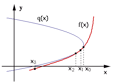
The inverse quadratic interpolation

Similar to the secant method that approximates the given function $f(x)$ by a straight line that goes through two consecutive points $\{x_n,\;f(x_n)\}$ and $\{x_{n-1},\;f(x_{n-1})\}$, the inverse quadratic interpolation method approximates the function by a quadratic curve that goes through three consecutive points $\{x_i,\;f(x_i)),\;\;(i=n,\;n-1,\;n-2)\}$. As the function may be better approximated by a quadratic curve rather than a straight line, the iteration is likely to converge more quickly.

In general, any function $y=f(x)$ can be approximated by a quadratic function $q(x)$ based on three points at $y_0=f(x_0)$, $y_1=f(x_1)$, and $y_2=f(x_2)$ by the Lagrange interpolation:

$$y=q(x)=\frac{(x-x_1)(x-x_2)}{(x_0-x_1)(x_0-x_2)}y_0 +\frac{(x-x_0)(x-x_2)}{(x_1-x_0)(x_1-x_2)}y_1 +\frac{(x-y_0)(x-x_1)}{(x_2-x_0)(x_2-x_1)}y_2$$ (33)

However, here we use the interpolation $x=q^{-1}(y)$ to approximate the inverse (horizontal) function $x=f^{-1}(y)$:

$$x=q^{-1}(y)=\frac{(y-y_1)(y-y_2)}{(y_0-y_1)(y_0-y_2)}x_0 +\frac{(... ...0)(y-y_2)}{(y_1-y_0)(y_1-y_2)}x_1 +\frac{(y-y_0)(y-y_1)}{(y_2-y_0)(y_2-y_1)}x_2$$ (34)

Obviously when $y=0$, the corresponding $x$ is the zero-crossing of $x=q^{-1}(y)$:

$$x_3=q^{-1}(y)\big\vert _{y=0}=\frac{y_1y_2}{(y_0-y_1)(y_0-y_2)}x_0 +\frac{y_0y_2}{(y_1-y_0)(y_1-y_2)}x_1 +\frac{y_0y_1}{(y_2-y_0)(y_2-y_1)}x_2$$ (35)

which can be used as an estimate of the root $x^*$ of $y=f(x)$. This expression can then be converted into an iteration by which the next root estimate $x_{n+1}$ is computed based on the previous three estimates at $x_n$, $x_{n-1}$, and $x_{n-2}$.

Brent's method

Brent's method combines the bisection method, secant method, and the method of inverse quadratic interpolation. In the iteration, a set of conditions is checked so that only the most suitable method under the current situation will be chosen to be used in the next iteration.