Solving Linear Equation Systems

Consider a linear equation system of $M$ equations and $N$ variables:

$$\left\{\begin{array}{l} \sum_{j=1}^N a_{1j} x_j-b_1=0\\ \cdots \\ \sum_{j=1}^N a_{Mj} x_j-b_M=0\end{array}\right.$$ (1)

which can be expressed in matrix form:

$${\bf Ax}-{\bf b}={\bf0}$$ (2)

where

$${\bf A}=\left[\begin{array}{ccc} a_{11} & \cdots & a_{1N}\\ \vdot... ...\;\;\;\;\;\; {\bf b}=\left[\begin{array}{c}b_1\\ \vdots\\ b_M\end{array}\right]$$ (3)

In general, the existence and uniqueness of the solution ${\bf x}$ can be determined by the fundamental theorem of linear algebra based on the rank $R$ of the coefficient matrix ${\bf A}$. Here we only consider some speical cases:

• $R=N=M$, ${\bf A}$ is full rank square matrix, and its inverse ${\bf A}^{-1}$ exists. Then the system has a unique solution:

  $${\bf x}={\bf A}^{-1}{\bf b}$$ (4)

• $R=M<N$, the system is under-determined or under-constrained and there may exist multiple solutions.
• $R=N<M$, the system is over-determined or over-constrained and no solution exists. However, we can still find the optimal solution in the least-squares sense.

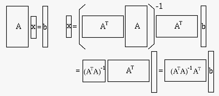
We now consider solving the over-determined linear system in last case. The error or residual of the ith equation is defined as $r_i=b_i-\sum_{j=1}^N a_{ij}x_j\;\;\;(i=1,\cdots,M)$, or in matrix form ${\bf r}={\bf b}-{\bf A}{\bf x}$ with ${\bf r}=[r_1,\cdots,r_M]^T$. The total sum-of-squares error of the system is:

$$\varepsilon({\bf x}) = \frac{1}{2}\sum_{i=1}^M r_i^2 =\frac{1}{2}\vert\vert{\bf r}\vert\... ...\bf r}^T{\bf r} =\frac{1}{2} ({\bf b}-{\bf A}{\bf x})^T({\bf b}-{\bf A}{\bf x})$$

$$= \frac{1}{2}\left( {\bf b}^T{\bf b}-{\bf x}^T{\bf A}^T{\bf b}-{\bf b}^T{\bf A}{\bf x}+{\bf x}^T{\bf A}^T{\bf A}{\bf x}\right)$$ (5)

To find the optimal solution ${\bf x}^*$ that minimizes $\varepsilon$, we set its derivative with respect to ${\bf x}$ to zero (see here):

$$\frac{d}{d{\bf x}}\varepsilon({\bf x}) = \frac{1}{2}\frac{d}{d{\bf x}}\vert\vert{\bf r}\vert\vert^2 =\frac... ...\bf A}^T{\bf b}-{\bf b}^T{\bf A}{\bf x}+{\bf x}^T{\bf A}^T{\bf A}{\bf x}\right)$$

$$= -{\bf A}^T{\bf b}+{\bf A}^T{\bf A}{\bf x}=0$$ (6)

and solve this matrix equation to get

$${\bf x}=\left({\bf A}^T{\bf A}\right)^{-1}{\bf A}^T{\bf b} ={\bf A}^-{\bf b}$$ (7)

where ${\bf A}^-=\left({\bf A}^T{\bf A}\right)^{-1}{\bf A}^T$ is the pseudo-inverse of the non-square matrix ${\bf A}$.

When the $M$ equations are barely independent, matrix ${\bf A}^T{\bf A}$ may be a near singular matrix with some eigenvalues close to zero, correspondingly its inverse $({\bf A}^T{\bf A})^{-1}$ may have some huge eigenvalues. Consequently the system may be ill-conditioned or ill-posed, in the sense that a small change in the system due to noise may cause a large change in the solution ${\bf x}$.

This problem can be addressed by regularization. Specificaly, by which the solution ${\bf x}$ is controled to not take unreasonably high values. Specifically we construct an objective function that contains a penalty term for large ${\bf x}$, as well as the error term $\varepsilon=\vert\vert{\bf r}\vert\vert^2/2$:

$$J({\bf x})=\frac{1}{2}\vert\vert{\bf r}\vert\vert^2+\frac{\lambda}{2}\vert\vert{\bf x}\vert\vert^2$$ (8)

By minimizing $J({\bf x})$, we can obtain a solution ${\bf x}$ of small norm $\vert\vert{\bf x}\vert\vert$ as well as low error $\varepsilon({\bf x})$. Same as before, the solution ${\bf x}$ can be obtained by setting the derivative of $J({\bf x})$ to zero

$$\frac{d}{d{\bf x}}J({\bf x})= -{\bf A}^T{\bf b}+{\bf A}^T{\bf Ax}+\lambda{\bf x}={\bf0}$$ (9)

and solving the resulting equation to get:

$${\bf x}=({\bf A}^T{\bf A}+\lambda{\bf I})^{-1}{\bf A}^T{\bf b}$$ (10)

We see that even if ${\bf A}^T{\bf A}$ is near singular, matrix ${\bf A}^T{\bf A}+\lambda{\bf I}$ is not due to the additional term $\lambda{\bf I}$.

By adjusting the hyperparameter $\lambda$, we can make a proper tradeoff between accuracy and stability.

• Small $\lambda$: the solution is more accurate but also more prone to noise and therefore less stable, i.e., the variance error may be large. This is called overfitting;
• Large $\lambda$: the solution is more stable as it is less affacted by noise, but it may be less accurate. This is called underfitting.

The issue of overfitting versus underfitting will be more formally addressed in a later chapter.