The Lagrange Interpolation

The polynomial $P_n(x)$ that fits a set of $n+1$ node points $\{x_i,\,y_i=f(x_i),\;i=0,\cdots,n\}$ can also be obtained by the Lagrange interpolation:

$$L_n(x)=\sum_{i=0}^n y_i l_i(x)$$ (15)

where $l_i(x)$ are the Lagrange basis polynomials of degree $n$ that span the space of all nth degree polynomials:

$$l_i(x)=\prod_{j=0,\;j\ne i}^n \frac{x-x_j}{x_i-x_j} =\frac{(x-x_0... ...{i+1})\cdots(x-x_n)} {(x_i-x_0)\cdots(x_i-x_{i-1})(x_i-x_{i+1})\cdots(x_i-x_n)}$$ (16)

Note that when $x=x_j,\;(j=0,\cdots,n)$, we get

$$l_i(x_j)=\delta_{ij}=\left\{\begin{array}{ll} 1 & i =j\\ 0 & i\ne j\end{array}\right.$$ (17)

This polynomial $L_n(x)$ passes through all $n+1$ points:

$$L_n(x_j)=\sum_{i=0}^n y_i l_i(x_j)=\sum_{i=0}^n y_i \delta_{ij} =y_j=f(x_j), \;\;\;\;\;\;(j=0,\cdots,n)$$ (18)

but it is only an approximation of $f(x)$ at any other point $x\ne x_j\;(j=0,\cdots,n)$.

Specially, when $f(x)=1$, i.e., $y_0=\cdots=y_n=1$, we get an important property of the Lagrange basis polynomials:

$$\sum_{i=0}^n l_i(x)=1$$ (19)

Due to the uniqueness of the polynomial interpolation, $L_n(x)=P_n(x)$, and they have the same error function as in Eq. (12):

$$f(x)-L_n(x)=R_n(x)=\frac{f^{(n+1)}(\xi)}{(n+1)!} l(x)$$ (20)

The computational complexity for calculating one of the $n$ basis polynomials $l_i(x),\; (i=0,\cdots,n)$ is $O(n)$ and the complexity for $L_n(x)$ is $O(n^2)$ for each $x$. If there are $m\gg n$ samples for $x$, then the total complexity is $O(n^2m)$.

To reduce the computational complexity, we express the numerator of $l_i(x)$ based on the (n+1)th degree polynomial $l(x)=\prod_{j=0}^n(x-x_j)$ defined in Eq. (7) as

$$\prod_{j=0,\;j\ne i}^n (x-x_j)=\frac{l(x)}{x-x_i}$$ (21)

Then the denominator of $l_i(x)$ can be found by evaluating $l(x)$ at $x=x_i$:

$$\prod_{j=0,\;j\ne i}^n(x_i-x_j) =\lim\limits_{x\rightarrow x_i}\p... ...0,\;j\ne i}^n(x-x_j) =\lim\limits_{x\rightarrow x_i}\frac{l(x)}{x-x_i} =l'(x_i)$$ (22)

Here the second to the last expression is an indeterminate form $0/0$ which leads to the last equality due to L'Hôpital's rule. Now the Lagrange basis polynomial can be expressed as

$$l_i(x)=\frac{l(x)}{(x-x_i)l'(x_i)}=l(x)\frac{w_i}{x-x_i}$$ (23)

where $w_i=1/l'(x_i)$ is the barycentric weight, and the Lagrange interpolation can be written as:

$$L_n(x)=\sum_{i=0}^n y_i l_i(x)=l(x)\sum_{i=0}^n y_i\frac{w_i}{x-x_i}$$ (24)

We see that the complexity for calculating $L_n(x)$ for each of the $m$ samples of $x$ is $O(n)$ (both for $l(x)$ and the summation), and the total complexity for all $m$ samples is $O(nm)$.

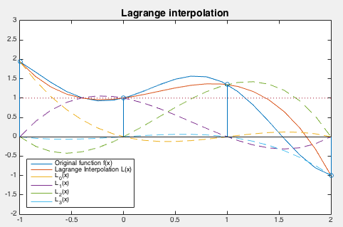
Example: Approximate function $y=f(x)=x\,\sin(2x+\pi/4)+1$ by a polynomial $p_n$ of degree $n=3$, based on the following $n+1=4$ points:

$$\begin{tabular}{c\vert\vert c\vert c\vert c\vert c}\hline i & 0 &... ...hline $y_i=f(x_i)$\ & 1.937 & 1.000 & 1.349 & -0.995 \\ \hline \end{tabular}\\$$

Based on these points, we construct the Lagrange polynomials as the basis functions of the polynomial space (instead of the power functions in the previous example):

$$l_0(x) = \frac{(x-0)(x-1)(x-2)}{-6}=\frac{x^3-3x^2+2x}{-6}$$

$$l_1(x) = \frac{(x+1)(x-1)(x-2)}{2}=\frac{x^3-2x^2-x+2}{2}$$

$$l_2(x) = \frac{(x+1)(x-0)(x-2)}{-2}=\frac{x^3-x^2-2x}{-2}$$

$$l_3((x) = \frac{(x+1)(x-0)(x-1)}{6}=\frac{x^3-x}{6}$$

Note that indeed $l_0(x)+l_1(x)+l_2(x)+l_3(x)=1$. The interpolating polynomial can be obtained as a weighted sum of these basis functions:

$$L_3(x)=1.937\;l_0(x)+1.0\;l_1(x)+1.349\;l_2(x)-0.995\;l_3(x) =1.0+0.369\,x+0.643\,x^2-0.663\,x^3 \\$$

which is the same as $P_3(x)$ previously found based on the power basis functions, with the same error $\epsilon=0.3063$.

The Matlab code that implements the Lagrange interpolation (both methods) is listed below:

function [v L]=LI(u,x,y)  % Lagrange Interpolation
    % vectors x and y contain n+1 points and the corresponding function values
    % vector u contains all discrete samples of the continuous argument of f(x)
    n=length(x);     % number of interpolating points
    k=length(u);     % number of discrete sample points
    v=zeros(1,k);    % Lagrange interpolation 
    L=ones(n,k);     % Lagrange basis polynomials
    for i=1:n
        for j=1:n
            if j~=i
                L(i,:)=L(i,:).*(u-x(j))/(x(i)-x(j));
            end
        end
        v=v+y(i)*L(i,:);
    end
end

function [v L]=LInew(u,x,y)  % Lagrange interpolation
    % u: data points; (x,y) sample points 
    n=length(x);     % number of sample points
    m=length(u);     % number of data points
    L=ones(n,m);     % Lagrange basis polynomials
    v=zeros(1,m);    % interpolation results
    w=ones(1,m);     % omega(x)
    dw=ones(1,n);    % omega'(x_i)
    for i=1:n
        w=w.*(u-x(i));
        for j=1:n
            if j~=i
                dw(i)=dw(i)*(x(i)-x(j));
            end
        end
    end
    for i=1:n
        L(i,:)=w./(u-x(i))/dw(i);
        v=v+y(i)*L(i,:);
    end
end