Value Function Approximation

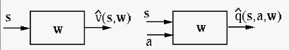
All previoiusly considered algorithms are based on either the state values function $v_\pi(s)$ for each state $s$ or the action value $q_\pi(s,a)$ for each state-action pair. As these function values can be considered as either a 1-D or 2-D table, the algorithms based on such function values are called tabular methods. However, when the number of states and the number of actions in each state are large (e.g., the game Go has $10^{170}$ states), the tabular methods are no longer suitable due to the unrealistic table sizes. In such a case, we can consider approximating the state value function $v(s)$ or action-value function $q(s,a)$ by a function $\hat{v}(s,{\bf w})$ or $\hat{q}(s,a,{\bf w})$, parameterized by a set of parameters as the components of vector ${\bf w}$. By doing so the state or action value functions can be represented more conveniently in terms of a much smaller number of parameters in ${\bf w}$.

This approach can be considered as a regression problem to fit a continuous function $\hat{v}(s,{\bf w})$ or $q(s,a,{\bf w})$ to a set of discrete and finite data points $v_\pi(s)$ or $q_\pi(s,a)$ obtained by sampling the MDP of the environment, so that all points in the state space, including those for stataes or state-action pairs never actually observed during the sampling process can be represented.

Examples of such value function approximators include

• linear combination of all features
• multi-layer neural networks
• decision trees

Same as in regression problems, we desire to find the optimal parameter ${\bf w}$ for the modeling function $\hat(v)_\pi(s,{\bf w})$ so that the following objective function, the mean squared error between the approximated values and the sample values, is minimized:

$$J({\bf w})=\frac{1}{2}E_\pi[(v_\pi(s)-\hat{v}(s,{\bf w}))^2 ]$$ (72)

where the expectation $E_\pi$ is with respect to all states visited while following some policy $\pi$. The gradient vector of $J({\bf w})$ is

$$\triangledown J({\bf w}) = \frac{d}{d{\bf w}}J({\bf w}) =\frac{1}{2}E_\pi\left[\frac{d}{d{\bf w}} \left[(v_\pi(s)-\hat{v}(s,{\bf w}))^2 \right]\right]$$

$$= -E_\pi\left[ (v_\pi(s)-\hat{v}(s,{\bf w})) \triangledown \hat{v}(s,{\bf w})\right]$$ (73)

and the optimal parameter vector ${\bf w}^*$ can be found iteratively by the gradient descent method

$${\bf w}_{n+1}={\bf w}_n+\Delta{\bf w} ={\bf w}_n-\alpha\triangled... ...\pi \left[ (v_\pi(s)-\hat{v}(s,{\bf w})) \triangledown\hat{v}(s,{\bf w})\right]$$ (74)

where $\alpha$ is the step size or learning rate, and

$$\Delta{\bf w}=-\alpha\triangledown{\bf J}({\bf w}) =\alpha E_\pi\left[ (v_\pi(s)-\hat{v}(s,{\bf w})) \triangledown \hat{v}(s,{\bf w})\right]$$ (75)

If the method of stochastic gradient descent (SGD) is used, i.e., the parameter ${\bf w}$ is updated based on only one data point at each iteration instead of the expectation of the data points, then $E_\pi$ for the expectation can be dropped:

$${\bf w}_{n+1}={\bf w}_n+\Delta{\bf w} ={\bf w}_n+ \alpha (v_\pi(s)-\hat{v}(s,{\bf w})) \triangledown \hat{v}(s,{\bf w}) )$$ (76)

Here the true value function $v_\pi(s)$, the expected return, is unknown and needs to be estimated by the actual return $G_t$ at each state $s=s_t$ based on the MC method, or $r_{t+1}+\gamma \hat{v}_\pi(s',{\bf w})$ in terms of the immediate reward $r_{t+1}$ and the estimated value $\hat{v}_\pi(s',{\bf w})$ of the next state $s'$ based on the TD method, by sampling the environment. Such an approach can be considered as a supervised learning based on labeled training data set: $\{ (s_t,\,G_t),\;\forall t\}$ for the MC method, or $\{ (s_t,\,r_{t+1},\;\forall t\}$ for xthe TD method.

In the following, we will consider the special case where the state value $v_\pi(s)$ is approximated by a linear function

$$\hat{v}(s,{\bf w})=\sum_{i=1}^d x_i w_i ={\bf w}^T{\bf x}(s)$$ (77)

based on the assumption that the value function of each state can be approximated as a linear combinatioin of a set of features in the feature vector ${\bf x}(s)=[x_1(s),\cdots,x_d(s)]^T$ for state $s$, weighted by the corresponding weights in the weight vector ${\bf w}=[w_1,\cdots,w_d]^T$ for all states.

As a simple example, if we represent each of the $N=\vert S\vert$ states $s_n$ by a $d=N$ dimensional binary feature vector ${\bf x}(s_n)=[x_1(s_n),\cdots,x_N(s_n)]^T$ of all zero components $x_i(s_n)=0$ except the n-th one $x_n(s_n)=1$, then the weight vector can be ${\bf w}=[w_1,\cdots,w_N]^T=[v_\pi(s_1),\cdots,v_\pi(s_N)]^T$, and we have $\hat{v}_\pi(s_n,{\bf w})={\bf w}^T{\bf x}(s_n)=v_\pi(s_n)$. In this case, each state $s$ is represented by its value function $v_\pi(s)$, same as in all previous discussions.

The objective function for the mean squared error of such a linear approximating function is

$$J({\bf w})=\frac{1}{2}E_\pi [(v_\pi(s)-\hat{v}(s,{\bf w}))^2 ] =\frac{1}{2}E_\pi[ (v_\pi(s)-{\bf w}^T{\bf x}(s))^2 ]$$ (78)

and its gradient is

$$\triangledown J({\bf w})=\frac{d}{d{\bf w}}J({\bf w}) =-E_\pi\left[ (v_\pi(s)-{\bf w}^T{\bf x}(s)) {\bf x}(s)\right]$$ (79)

If all data points in terms of state $s$ represented by ${\bf x}(s)$ and the corresponding return $G(s)$ as a sample of the true value $v_\pi(s)$ have already been collected, then the value function approximation can be carried out as an off-line algorithm in a batch manner, the same as in the linear least squares linear regression problem discussed in a previous chapter, and the optimal weight vector that minimizes the squared error

$${\bf w}^*=\argmax_{\bf x} \sum_s [G(s)-\hat{v}_\pi(s,{\bf w})]^2$$ (80)

can be found by the same pseudo inverse method

$${\bf w}^*=({\bf XX}^T)^{-1}{\bf XG}$$ (81)

where ${\bf X}=[{\bf x}_1,\cdots,{\bf x}_N]$ is a matrix containing all $N$ samples for the states and ${\bf G}=[G_1,\cdots,G_N]^T$ is a vector containing the corresponding returns.

However, as reinforcement learning is typically an online problem, the parameter ${\bf w}$ for the approximator needs to be modified in real-time whenever a new piece of data becomes available during the sampling of the environment. In this case, we can find the gradient descent method, based on the gradient vector of $J({\bf w})$:

$$\triangledown J({\bf w}) = \frac{d}{d{\bf w}}J({\bf w}) =-E_\pi(v_\pi(s)-\hat{v}(s,{\bf w})) \triangledown \hat{v}(s,{\bf w})$$

$$= -E_\pi(v_\pi(s)-{\bf w}^T{\bf x}(s)){\bf x}(s)$$ (82)

and the optimal parameter ${\bf w}^*$ can be found iteratively

$${\bf w}_{n+1} = {\bf w}_n+\Delta{\bf w}={\bf w}_n+\alpha E_\pi\left[v_\pi(s)-\hat{v}(s,{\bf w})\right] \triangledown \hat{v}(s,{\bf w})$$

$$= {\bf w}_n+\alpha E_\pi\left[v_\pi(s)-{\bf w}^T{\bf x}(s) \right]{\bf x}(s)$$ (83)

where $\Delta{\bf w}$ is the increment in each iteration:

$$\Delta{\bf w} =\alpha E_\pi\left[v_\pi(s)-\hat{v}(s,{\bf w})\righ... ...s,{\bf w}) =\alpha E_\pi\left[v_\pi(s)-{\bf w}_n^T{\bf x}(s) \right] {\bf x}(s)$$ (84)

If stochastic gradient descent is used, then ${\bf w}$ is updated whenever a new sample data point ${\bf x}(s_t)$ is available at a time step $t$, then the expectation $E_\pi$ in the equations above can be dropped.

We note that the expectation of the estimated ${\bf w}$ found by this SGD method is the same as that obtained by full GD method. Also this iteration will convergence to the global minimum of the objective function $J({\bf w})$ in Eq. (78) as it is a quadratic function with only one minimum which is global.

Specifically, the state value function is unknown and can be estimated in several different ways, similar to the corresponding algorithms discussed before.

• MC method

  The value function $v_\pi(s)$ is estimated by the actual return $G_t$ for each state $s_t$ visited in an episode, obtained only at the end of each episode while sampling the environment:

  $$\Delta{\bf w}=\alpha[G_t-\hat{v}(s_t,{\bf w})] \triangledown \hat{v}(s_t,{\bf w}) =\alpha[G_t-{\bf w}^T{\bf x}(s_t)]{\bf x}(s_t)$$ (85)

  Here is the pseudo code for the algorithm based on the MC method, similar to that for value evaluation algorithms discussed previously:

  Initialize ${\bf w}={\bf0}$

  loop (for each episode)

  run current episode to the end to get $G_t,\;t=1,\cdots,T$

  for $t=1,\cdots,T$

  if $s_t$ is visited the first time

  ${\bf w}={\bf w}+\alpha[G_t-{\bf w}^T{\bf x}(s_t)] {\bf x}(s_t)$

  end if

  end for

  end loop

• TD(0) method

  The value function $v_\pi(s)$ is estimated by the TD target, the sum of the immediate reward $r_{t+1}$ and the approximated value of the next state $s_{t+1}$, at each time step of each episode while sampling the environment:

  $$\Delta{\bf w}=\alpha[r_{t+1}+\gamma {\bf w}^T{\bf x}(s_{t+1}) -{\bf w}^T{\bf x}(s_t)] {\bf x}(s_t)$$ (86)

  Here is the pseudo code for the algorithm based on the TD method, similar to that for value evaluation algorithms discussed previously:

  Initialize ${\bf w}={\bf0}$

  loop (for each episode)

  for each time step in current episode

  take action $a=\pi(s)$, get reward $r$ and next state $s'$

  ${\bf w}={\bf w}+\alpha[r+\gamma {\bf w}^T{\bf x}(s')-{\bf w}^T{\bf x}(s)]{\bf x}(s)$

  end for

  end loop

• TD($\lambda$) method

  The value function $v_\pi(s)$ is estimated based on $\lambda$-return $G_t^\lambda$ given in Eq. (62). As discussed before, TD($\lambda$) has two flavors:

  • Forward veiw: same as MC method, except the true return $G_t$ is replaced by $\lambda$-return $G_t^\lambda$ available only at the end of each spisode:

    $$\Delta{\bf w}=\alpha[G_t^{\lambda}-{\bf w}^T{\bf x}(s_t)] {\bf x}(s_t)$$ (87)

  • Backward view: similar to TD(0), this is based on the immediate reward $r_{t+1}$ available at every step of each episode:

    $$\delta_t=\alpha[r_{t+1}+\gamma{\bf w}^T{\bf x}(s_{t+1})-{\bf w}^T{\bf x}(s_t)] {\bf x}(s_t)$$ (88)

    $$e_t=\gamma\lambda e_{t-1}+{\bf x}(s_t),\;\;\;\;\;\; \Delta{\bf w}=\alpha\delta_t e_t$$ (89)

Given a policy $\pi$ for an MDP, we define a probability districution $d(s)$ over all staes visited according to $\pi$, satisfying

$$\sum_s d(s)=1$$ (90)

and the following balance equation:

$$d(s')=\sum_s\sum_a \pi(a\vert s)p(s'\vert s,a)d(s)$$ (91)

As both $d(s')$ and $d(s)$ represent the same distribution, they must be identical.

Given the probability distribution $d(s)$, the mean squared error of the value function approximation for a policy $\pi$ can be expressed as

$$MSE({\bf w})=\sum_s d(s)[v_\pi(s)-\hat{v}_\pi(s,{\bf w})]^2$$ (92)

It can be shown that the MC method for the linear value function approximation will converge to the optimal weight vector ${\bf w}_{MC}$ that minimizes the mean squared error above:

$$MSE({\bf w}_{MC})=\min_{\bf w} \sum_s d(s)[v_\pi(s)-\hat{v}_\pi(s,{\bf w})]^2$$ (93)