Real and Reactive Power and Power Factor

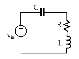
All loads of a power plant can be modeled by a two-terminal network of passive elements (resistors, inductors, capacitors, without any energy sources) with a total complex impedance

$$Z=R+jX=\vert Z\vert e^{j\angle Z}=\vert Z\vert e^{j\phi},\;\;\;\;... ...\vert Z\vert=\sqrt{R^2+X^2}\\ \angle Z=\phi=\tan^{-1}(X/R)>0 \end{array}\right.$$ (391)

As the loads are typically inductive (e.g., electric motors, transformers), i.e., $X=\omega L>0$, the phase angle $\phi=\angle Z$ of the impedance is positive. We are concerned with the energy consumption (by $R$) and storage (in $L$) in the load. Let the input voltage to the load network be:

$$v(t)=\sqrt{2}V_{rms} \cos(\omega t),\;\;\;\;\dot{V}=\sqrt{2}V_{rms}\angle 0$$ (392)

then the current through the power transmission line and load can be found:

$$\dot{I}=\frac{\dot{V}}{Z}=\frac{\sqrt{2}V_{rms}}{\vert Z\vert\ang... ... =\sqrt{2}I_{rms}\angle(-\phi),\;\;\;\;i(t)=\sqrt{2}I_{rms} \cos(\omega t-\phi)$$ (393)

where $I_{rms}=V_{rms}/\vert Z\vert$ is the RMS or effective value of the current. Note that the current is lagging the voltage by an angle $\phi$.

Consider the instantaneous power of the load defined as the product of the voltage and current:

$$p_{in}(t) = v(t)\;i(t)=\sqrt{2}V_{rms}\cos(\omega t)\;\sqrt{2}I_{rms}\cos(\omega t-\phi)$$

$$= 2V_{rms}I_{rms}\;\cos(\omega t)\;[\cos(\omega t)\cos\phi +\sin(\omega t)\sin\phi ]$$

$$= V_{rms}I_{rms} \left[\cos\phi\, \left(2\cos^2(\omega t)\right) +\sin\phi\,\left(2\cos(\omega t)\sin(\omega t)\right) \right]$$

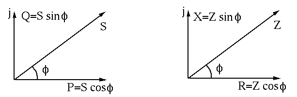
$$= V_{rms}I_{rms} \;\left[ \cos\phi\; p(t) + \sin\phi\; q(t) \right]$$

$$= S \;\left[\cos\phi\; p(t) + \sin\phi\; q(t) \right] =P\; p(t)+Q\; q(t)$$ (394)

where we have defined

$$p(t)=2\cos^2(\omega t)=1+\cos 2\omega t,\;\;\;\;\;\; q(t)=2\cos(\omega t)\sin(\omega t)=\sin 2\omega t$$ (395)

and

• Apparent Power (in volt-amperes): $S=V_{rms}I_{rms}$
• Real power (in Watts): $P=S\cos\phi$ as the
• Reactive power (in volt-ampere reactive or VAR): $Q=S\sin\phi$

The plots below show that the instantaneous power $p_{in}(t)$ can be represented as either a product of $v(t)$ and $i(t)$, or a weighted sum of the real power $p(t)$ and reactive power $q(t)$.

We note that

$$\frac{1}{T}\int_T p(t)dt=\frac{1}{T}\int_T [1+cos(2\omega t)] dt=1 \;\;\;\;\;\; \frac{1}{T}\int_T q(t)dt=\frac{1}{T}\int_T \sin(2\omega t) dt=0$$ (396)

Consider the average power over one period $T=2\pi/\omega$:

$$P_{average} = \frac{1}{T}\int_T p_{in}(t)dt =\frac{1}{T}\int_T \left[P\; p(t) + Q\; q(t) \right] dt$$

$$= S\cos\phi\;\frac{1}{T}\int_T p(t)dt+S\sin\phi\;\frac{1}{T}\int_T q(t)dt$$

$$= P\;1+Q\;0=P$$ (397)

We see that

• The real power $P=S\cos\phi$ represents the average power dissipation by the load over one period $T$;
• The reactive power $Q=S\sin\phi$ is not consumed but converted back and forth between the energy source and the energy storing (inductive) elements in the load.

The apparent power $S=V_{rms}I_{rms}$ can be considered as the magnitude of a complex product of $\dot{V}=V_{rms}\angle 0$ and $\overline{\dot{I}}=\overline{I_{rms}\angle(-\phi)}=I_{rms}\angle\phi$:

$$\dot{V}\overline{\dot{I}}=V_{rms}\angle 0\; I_{rms}\angle \phi=V_{rms}I_{rms}\angle \phi =S(\cos\phi+j\;\sin\phi)=P+jQ$$ (398)

On the other hand, as $\dot{V}=Z\dot{I}=(R+jX)\dot{I}$, the above can also be written as:

$$\dot{V}\overline{\dot{I}}=Z\dot{I}\overline{\dot{I}} =(R+jX)\dot{I}\overline{\dot{I}}=RI^2_{rms}+jX I^2_{rms}$$ (399)

Comparing the two expressions of $\dot{V}\overline{\dot{I}}$ above, we get:

$$\left\{ \begin{array}{l} P=I^2_{rms}R=S\;\cos\phi \\ Q=I^2_{rms}X=S\;\sin\phi \\ S=I^2_{rms}Z \end{array} \right.$$ (400)

the last equation is due to

$$S^2=P^2+Q^2=I^4_{rms}(R^2+X^2)=I^4_{rms}Z^2=(I^2_{rms}Z)^2$$ (401)

We see that

• The apparent power is $S=I^2_{rms}Z$;
• The real power is $P=I^2_{rms}R$, which is dissipated by the resistive component $R$ of the load;
• The reactive power is $Q=I^2_{rms}X$, which is stored in and released from the reactive component $L$ of the load.

Improvement of Power Factor

The Power factor is defined as

$$\lambda\stackrel{\triangle}{=}\cos \phi < 1$$ (402)

It is desirable to maximize the power factor $\lambda$ by reducing $\phi$, for higher efficiency of the power transmission system, i.e., to deliver the real power $P$ to the load with minimum reactive power $Q$ (thereby minimum current and power dissipation along the transmission line).

To do so, we can include a shunt capacitor $C$ to cancel the inductive effect in the system, thereby reducing $\phi$ and increasing $\lambda$.

The most straight forward way is to add the shunt capacitor $C=1/\omega L$ in series with the inductive load, so that the inductive reactance $j\omega L$ is completely canceled by the capacitive reactance $1/j\omega C=-j\omega L$.

However, we also note that at resonance, the voltages across $L$ and $C$ are $Q$ times the voltage across $R$, which is the same as the source voltage (see this page):

$$\dot{V}_L=jQ\dot{V}_R,\;\;\;\;\;\dot{V}_C=-jQ\dot{V}_R$$ (403)

the voltage across the inductive load $R+j\omega L$ becomes $\dot{V}_{RL}=\dot{V}_L+\dot{V}_R=jQ\dot{V}+\dot{V}=(1+jQ)\dot{V}$, which could be much higher than the expected source voltage $\dot{V}$ (without capacitor $C$) if $Q$ is large. Consequently, improper operation of the load or even damage may result.

The right way to compensate for the inductive impedance of the circuit is to include the shunt capacitor $C$ in parallel to the inductive load so that it still gets the expected voltage.

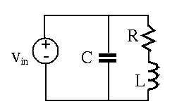
Now the overall load becomes

$$Z_{total} = Z_{RL}\vert\vert Z_C=(R+j\omega L)\; \vert\vert \;(1/j\omega C)$$

$$= \frac{(R+j\omega L)/j\omega C}{(R+j\omega L)+1/j\omega C} =\frac{R+j\omega L}{j\omega CR-\omega^2 LC+1}$$ (404)

We need to find the capacitance $C$ so that the new phase angle $\phi=\angle Z_{total}$ is zero, i.e., the phases of the numerator and denominator need are the same:

$$\tan^{-1}\left(\frac{\omega L}{R}\right) =\tan^{-1}\left(\frac{\omega RC}{1-\omega^2 LC}\right), \;\;\;\;\; \;\;\;\;\;\; \frac{\omega L}{R}=\frac{\omega RC}{1-\omega^2 LC} \;\;\;\;\; \;\;\;\;\;\; L-\omega^2 L^2C=R^2C$$ (405)

Solving this equation for $C$ we get:

$$C_p=\frac{L}{R^2+\omega^2 L^2} =\frac{1}{R^2/L+\omega^2 L}<\frac{1}{\omega^2L}=C_s$$ (406)

Now the voltage across the inductive load is still the same as the voltage source as expected, and another benefit is that the required capacitance $C_p$ is smaller than the capacitance $C_s=1/\omega^2 L$ required for the series approach.

Power factor correction

Shunt capacitors

To reduce the cost of a large capacitance needed for the phase angle of the load to be reduced to zero $\phi=0$ so that $\lambda=\cos\phi=1$, it is acceptable for the improved power factor to be less than 1, e.g., 0.95. In this case, the phase angle of the load is

$$\phi=\angle Z'=\tan^{-1}\left(\frac{\omega L}{R}\right)-\tan^{-1}\left(\frac{\omega RC}{1-\omega^2 LC}\right)=\cos^{-1}\; 0.95=18.2^\circ$$ (407)

Solving this equation for $C$ we get the required capacitance. As now we have

$$\tan^{-1}\left(\frac{\omega L}{R}\right)>\tan^{-1}\left(\frac{\omega RC}{1-\omega^2 LC}\right)$$ (408)

i.e.,

$$\frac{\omega L}{R}>\frac{\omega RC}{1-\omega^2 LC}$$ (409)

we get an even smaller capacitance which is more practically implementable:

$$C<\frac{L}{R^2+\omega^2 L^2}=\frac{1}{R^2/L+\omega^2L}$$ (410)