Sequential Minimal Optimization (SMO) Algorithm

The sequential minimal optimization (SMO, due to John Platt 1998, also see notes here) is a more efficient algorithm for solving the SVM problem, compared with the generic QP algorithms such as the internal-point method. The SMO algorithm can be considered as a method of decomposition, by which an optimization problem of multiple variables is decomposed into a series of subproblems each optimizing an objective function of a small number of variables, typically only one, while all other variables are treated as constants that remain unchanged in the subproblem. For example, the coordinate descent algorithm is just such a decomposition method, which solves a problem in a multi-dimensional space by converting it into a sequence of subproblems each in a one-dimensional space.

When applying the decomposition method to the soft margin SVM problem, we could consider optimizing only one variable $\alpha_i$ at a time, while treating all remaining variables $\alpha_1,\cdots,\alpha_{i-1},\alpha_{i+1},\cdots,\alpha_N$ as constants. However, due to the constraint $\sum_{n=1}^N \alpha_n y_n=0$, $\alpha_i$ is a linear combination of $N-1$ constants and is therefore also a constant. We therefore need to consider two variables at a time, here assumed to be $\alpha_i$ and $\alpha_j$, while treating the remaining $N-2$ variables as constants. The objective function of such a subproblem can be obtained by dropping all constant terms independent of the two selected variables $\alpha_i$ and $\alpha_j$ in the original objective function in Eq. (131):

$$\;\; L(\alpha_i,\alpha_j) =\alpha_i+\alpha_j-\frac{1}{2}\left( \alpha_... ...pha_j^2{\bf x}_j^T{\bf x}_j +2\alpha_i\alpha_jy_iy_j{\bf x}_i^T{\bf x}_j\right)$$

$$-\alpha_iy_i\left(\sum_{n\ne i}\alpha_ny_n{\bf x}_n^T\right){\bf x}_i -\alpha_jy_j\left(\sum_{n\ne j}\alpha_ny_n{\bf x}_n^T\right){\bf x}_j$$

$$= \alpha_i+\alpha_j-\frac{1}{2}\left(\alpha_1^2 K_{ii}+\alpha_2^2K_{jj} +2\alpha_i\alpha_jy_iy_jK_{ij}\right)$$

$$-\alpha_iy_i\sum_{n\ne i,j}\alpha_ny_nK_{ni} -\alpha_jy_j\sum_{n\ne i,,j}\alpha_ny_nK_{nj}$$

$$\;\; 0\le\alpha_i,\alpha_j\le C,\;\;\;\;\;\; \sum_{n=1}^N \alpha_ny_n=0$$ (135)

where, to use the kernel method, all inner products ${\bf x}_m^T{\bf x}_n$ are replaced by the corresponding kernel function $K_{mn}=K({\bf x}_m,{\bf x}_n)={\bf z}_m^T{\bf z}_n$ with ${\bf z}_n=\phi({\bf x}_n)$.

This maximization problem can be solved iteratively. Out of all previous values $\alpha_n^{old}\,(n=1,\cdots,N)$, the two selected variables are updated to their correspoinding new values $\alpha_i^{new}$ and $\alpha_j^{new}$ that maximize $L(\alpha_i,\alpha_j)$, subject to the two constraints.

We rewrite the second constraint as

$$\alpha_iy_i+\alpha_jy_j=-\sum_{n\ne i,j} \alpha_ny_n$$ (136)

and multiply both sides by $y_i$ to get

$$y_i^2\alpha_i+y_iy_j\alpha_j=\alpha_i+s\alpha_j =\left(-\sum_{n\ne i,j} \alpha_ny_n\right)y_i =\delta,\;\;\;\;\; \;\;\;\;\;\alpha_i=\delta-s\alpha_j$$ (137)

where we have defined $s=y_iy_j$ and $\delta=-\sum_{n\ne i,j} \alpha_ny_ny_i$. As $\delta$ is independent of $\alpha_i$ and $\alpha_j$, it remains the same before and after they are updated, and we have

$$\alpha_i^{new}+s\alpha_j^{new}=\alpha_i^{old}+s\alpha_j^{old}=\delta$$ (138)

i.e.,

$$\Delta\alpha_i=\alpha_i^{new}-\alpha_i^{old} =-s(\alpha_j^{new}-\alpha_j^{old})=-s\Delta\alpha_j$$ (139)

We now consider a closed-form solution for updating $\alpha_i$ and $\alpha_j$ in each iteration of this two-variable optimization problem. We first rewrite Eq. (86) as

$$\sum_{n\ne i,j}\alpha_ny_n{\bf x}_n ={\bf w}-\alpha_iy_i{\bf x}_i-\alpha_jy_j{\bf x}_j$$ (140)

so that the two summations in $L(\alpha_i,\alpha_j)$, now denoted by $v_k\;(k=i,j)$, can be written as

$$v_k = \sum_{n\ne i,j}\alpha_ny_nK_{nk} =\sum_{n=1}^N\alpha_ny_nK_{nk}-\alpha_iy_iK_{ik}-\alpha_jy_jK_{jk}$$

$$= \left(\sum_{n=1}^N\alpha_ny_nK_{nk}+b\right) -b-\alpha_iy_iK_{ik}-\alpha_jy_jK_{jk}$$

$$= u_k-b-\alpha_iy_iK_{ik}-\alpha_jy_jK_{jk}$$ (141)

where

$$u_k=f({\bf z}_k)=\sum_{n=1}^N\alpha_ny_nK_{nk}+b$$ (142)

is the output in Eq. (114) corresponding to input ${\bf x}_k$. Now the objective function above can be written as:

$$L(\alpha_i,\alpha_j) = \alpha_i+\alpha_j-\frac{1}{2} (\alpha_i^2 K_{ii}+\alpha_j^2K_{jj} +2s\alpha_i\alpha_jK_{ij})-\alpha_iy_iv_i-\alpha_jy_jv_j$$ (143)

Substituting $\alpha_i=\delta-s\alpha_j$ (Eq. (139)) into $L(\alpha_i,\alpha_j)$, we can rewrite it as a function of a single variable $\alpha_j$ alone:

$$L(\alpha_j) = \delta+(1-s)\alpha_j -\frac{1}{2}\left[ (\delta-s\alpha_j)^2K_{ii} +\alpha_j^2K_{jj}+2s(\delta-s\alpha_j)\alpha_jK_{ij}\right]$$

$$-(\delta-s\alpha_j)y_iv_i-\alpha_jy_jv_j$$

$$= \frac{1}{2}(2K_{ij}-K_{ii}-K_{jj})\alpha_j^2 +[1-s+s\delta(K_{ii}-K_{ij})+y_j(v_i-v_j)]\alpha_j+$$ (144)

where $s^2=(y_iy_j)^2=1$, and scalar Const. represents all constant terms independent of $\alpha_i$ and $\alpha_j$ and can therefore be dropped. Now the objective function becomes a quadratic function of the single variable $\alpha_j$. Consider the coefficients of this quadratic function:

• The coefficient of $\alpha_j^2$:

  $$\frac{1}{2}(2K_{ij}-K_{ii}-K_{jj})=\frac{1}{2}\eta$$ (145)

  where $\eta$ is defined as
  

  $$\eta = 2K_{ij}-K_{ii}-K_{jj} =2{\bf z}_i^T{\bf z}_j-{\bf z}_i^T{\bf z}_i-{\bf z}_j^T{\bf z}_j =-({\bf z}_i-{\bf z}_j)^T({\bf z}_i-{\bf z}_j)$$

  $$= -\vert\vert{\bf z}_i-{\bf z}_j\vert\vert^2\le 0$$ (146)

  
  
• The coefficient of $\alpha_j$:
  

  $$1-s+s\delta(K_{ii}-K_{ij})+y_j(v_i-v_j)$$

  $$= 1-s+(s\alpha_i+\alpha_j)(K_{ii}-K_{ij})$$

  $$+y_j[(u_i-b-\alpha_iy_iK_{ii}-\alpha_jy_jK_{ij})- (u_j-b-\alpha_iy_iK_{ij}-\alpha_jy_jK_{jj})]$$

  $$= 1-s+s\alpha_1(K_{ii}-K_{ij})+\alpha_2(K_{ii}-K_{ij})$$

  $$+y_j(u_i-u_j)-\alpha_isK_{ii}-\alpha_jK_{ij} +\alpha_isK_{ij}+\alpha_jK_{jj}$$

  $$= y_j^2-s-\alpha_j(2K_{ij}-K_{ii}-2K_{jj})+y_j(u_i-u_j)$$

  $$= y_j(u_i-y_j-u_j+y_j)-\alpha_j(2K_{ij}-K_{ii}-K_{jj})$$

  $$= y_j(E_i-E_j)-\alpha_j\eta$$ (147)

  
  where we have defined

  $$E_k=u_k-y_k=\sum_{n=1}^N\alpha^{old}_ny_nK_{nk}+b-y_k \;\;\;\;\;(k=1,2)$$ (148)

  as the difference between the desired output $y_k$ and the actual output based on the previous values of the variables $\alpha_n^{old}\;(n=1,\cdots,N)$.

Now the quadratic objective function can be rewritten as:

$$L(\alpha_j)=\frac{1}{2}\eta\alpha_j^2 +\left[y_j(E_i-E_j)-\alpha_j^{old}\eta\right]\alpha_j$$ (149)

Given the previous values $\alpha_n^{old}\;(n=1,\cdots,N)$ in the coefficients, we will find $\alpha_j^{new}$ that maximizes $L(\alpha_j)$. Consider its first and second order derivatives:

$$\frac{d}{d\alpha_j}L(\alpha_j) = \eta\alpha_j+y_j(E_i-E_j)-\alpha_j^{old}\eta$$

$$\frac{d^2}{d\alpha_j^2}L(\alpha_j) = \eta\le 0$$ (150)

As the second order derivative of $L(\alpha_j)$ is $\eta\le 0$, it has a maximum. Solving the equation $d\,L(\alpha_j)/d\alpha_j=0$, we get $\alpha_j^{new}$ that maximizes $L(\alpha_j)$ based on the old value $\alpha_j^{old}$:

$$\alpha_j^{new}=\alpha_j^{old}+\frac{y_j(E_j-E_i)}{\eta} =\alpha_j... ...;\;\;\; \Delta\alpha_j=\alpha_j^{new}-\alpha_j^{old}=\frac{y_j(E_j-E_i)}{\eta},$$ (151)

Note that this is an unconstrained solution, which needs to be modified if the constraints in Eq. (135) are violated. As shown in the figure below, $\alpha_i$ and $\alpha_j$ are inside the square of size $C$, due to the first constraint $0\le \alpha_i,\;\alpha_j\le C$; also, due to the second constraint $\alpha_i+s\alpha_j=\delta$ (Eq. (137)), they have to be on the diagonal line segment inside the square.

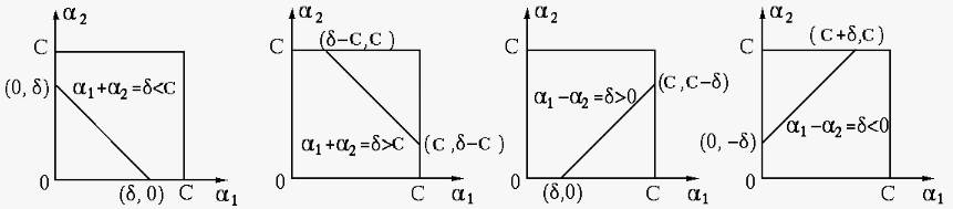
The four panels correspond to the four possible cases, depending on whether $s=1$ ( $y_i=y_j=\pm 1$, panels 1 and 2), or $s=-1$ ( $y_i=-y_j=\pm 1$, panels 3 and 4), and whether $\delta<C$ (panels 1 and 3) or $\delta>C$ (panels 2 and 4), which can be further summarized below in terms of the lower bound $L$ and upper bound $H$ of $\alpha_2$:

• If $s=1$, then $\alpha_i+s\alpha_j=\alpha_i+\alpha_j=\delta$,
  • if $\delta<C$, then $\min(\alpha_j)=0,\;\max(\alpha_j)=\delta$ (first panel)
  • if $\delta>C$, then $\min(\alpha_j)=\delta-C,\;\max(\alpha_j)=C$ (second panel)
  Combining these two cases, we have

  $$\left\{\begin{array}{l} L=\max(0,\;\delta-C)=\max(0,\;\alpha_i+\alpha_j-C)\\ H=\min(\delta,\;C)=\min(\alpha_i+\alpha_j,\;C) \end{array}\right.$$ (152)

• If $s=-1$, then $\alpha_i+s\alpha_j=\alpha_i-\alpha_j=\delta$,
  • if $\delta>0$, then $\min(\alpha_j)=0,\;\max(\alpha_j)=C-\delta$ (third panel)
  • if $\delta<0$, then $\min(\alpha_j)=-\delta,\;\max(\alpha_j)=C$ (fourth panel)
  Combining these two cases, we have

  $$\left\{\begin{array}{l} L=\max(0,\;-\delta)=\max(0,\;\alpha_j-\alpha_i)\\ H=\min(C-\delta,\;C)=\min(C+\alpha_j-\alpha_i,\;C) \end{array}\right.$$ (153)

Now we apply the constraints in terms of $L$ and $H$ to the optimial solution $\alpha_j^{new}$ obtained previously to get $\alpha_j$ that is feasible as well as optmal:

$$\alpha_j^{new}\Longleftarrow \left\{\begin{array}{cl} H & \mbox{i... ... } L<\alpha_2^{new} < H\\ L & \mbox{if } \alpha_j^{new}\le L\end{array}\right.$$ (154)

We can further find $\alpha_i$ based on Eq. (139):

$$\alpha_i^{new}=\alpha_i^{old}-s\Delta\alpha_j =\alpha_i^{old}-s(\alpha_j^{new}-\alpha_j^{old})$$ (155)

and update the weight vector based on Eq. (118):

$${\bf w}^{new} = \sum_{n\ne i,j} y_n\alpha_n^{old}{\bf x}_n +y_i\alpha_i^{new}{\bf x}_i+y_j\alpha_j^{new}{\bf x}_j$$

$$= {\bf w}^{old}-y_i\alpha_i^{old}{\bf x}_i-y_j\alpha_j^{old}{\bf x}_j +y_i\alpha_i^{new}{\bf x}_i+y_j\alpha_j^{new}{\bf x}_j$$

$$= {\bf w}^{old}+y_i\Delta\alpha_i{\bf x}_i+y_j\Delta\alpha_j{\bf x}_j ={\bf w}^{old}+\Delta{\bf w}$$ (156)

where $\Delta{\bf w}={\bf w}^{new}-{\bf w}^{old} =y_i\Delta\alpha_i{\bf x}_i+y_j\Delta\alpha_j{\bf x}_j$. To update $b$, consider:

$$\Delta E_k = E_k^{new}-E_k^{old}=u_k^{new}-u_k^{old}$$

$$= \sum_{n=1}^N\alpha_n^{new}y_nK_{nk}+b^{new} -\sum_{n=1}^N\alpha_n^{old}y_nK_{nk}-b^{old}$$

$$= y_i\Delta\alpha_iK_{ik}+y_j\Delta\alpha_jK_{jk} +b^{new}-b^{old} \;\;\;\;\;(k=1,2)$$ (157)

Consider the following cases:

• If $0<\alpha_k<C$ for either $k=i$ or $k=j$, then $y_kE_k=0$ according to Eq. (130). We let $E_k^{new}=0$ and solve the equation above to get:

  $$b^{new}_k=b^{old}_k-(E_k^{old}+y_i\Delta\alpha_iK_{ik}+y_j\Delta\alpha_jK_{jk}) \;\;\;\;\;(k=1\; \;2)$$ (158)

• If $0<\alpha_k<C$ for both $k=i$ and $k=j$, then $b_i^{new}=b_j^{new}$.
• If $\alpha_k=0$ or $\alpha_k=C$ for both $k=i$ and $k=2$, then $E_k\ne 0$, and $b^{new}_i\ne b^{new}_j$, their average $b^{new}=(b_i^{new}+b_j^{new})/2$ can be used.

The computation above for maximizing $L(\alpha_i,\alpha_j)$ is carried out iteratively each time when a pair of variables $\alpha_i$ and $\alpha_j$ is selected to be updated. Specifically, we select a variable $\alpha_i$ that violates any of the KKT conditions given in Eq. (130) in the outer loop of the SMO algorithm, and then pick a second variable $\alpha_j$ in the inner loop of the algorithm, both to be optimized. The selection of these variables can be either random (e.g., by following their order), or guided by some heuristics, such as always choosing the variable with maximum step size $\Delta\alpha_n=\alpha^{new}_n-\alpha^{old}_n$. This iterative process is repeated until convergence when the KKT conditions are satisfied by all $\alpha_1,\cdots,\alpha_N$ variables, i.e., no more variables need to be updated. All data points corresponding to $\alpha_n\ne 0$ are the support vectors, based on which we can find the offset $b$ by Eq. (133) and classify any unlabeled point ${\bf x}$ by Eq. (134).

The Matlab code for the essential part of the SMO algorithm is listed below, based mostly on a simplified SMO algorithm and the related code with some modifications.

In particular, the if-statement

 
if (alpha(i)<C & yE<-tol) | (alpha(i)>0 & yE>tol)

checks the three KKT conditions in Eq. (130), where $yE=y_nE_n$ and $tol$ is a small constant. The first half checks if the first two of the three conditions are violated, while the second half checks if the second two of the three conditions are violated.

    [X y]=getData;                       % get training data
    [m n]=size(X);                       % size of data
    alpha=zeros(1,n);                    % alpha variables
    bias=0;                              % initial bias
    it=0;                                % iteration index                
    while (it<maxit)                     % number of iterations less than maximum
        it=it+1;
        changed_alphas=0;                % number of changed alphas
        N=length(y);                     % number of support vectors
        for i=1:N                        % for each alpha_i
            Ei=sum(alpha.*y.*K(X,X(:,i)))+bias-y(i);    
            yE=Ei*y(i);
            if (alpha(i)<C & yE<-tol) | (alpha(i)>0 & yE>tol)   % KKT violation
                for j=[1:i-1,i+1:N]        % for each alpha_j not equal alpha_i
                    Ej=sum(alpha.*y.*K(X,X(:,j)))+bias-y(j);
                    ai=alpha(i);         % alpha_i old
                    aj=alpha(j);         % alpha_j old
                    if y(i)==y(j)        % s=y_i y_j=1
                        L=max(0,alpha(i)+alpha(j)-C);
                        H=min(C,alpha(i)+alpha(j));
                    else                 % s=y_i y_j=-1
                        L=max(0,alpha(j)-alpha(i));
                        H=min(C,C+alpha(j)-alpha(i));
                    end
                    if L==H              % skip when L==H
                        continue
                    end
                    eta=2*K(X(:,j),X(:,i))-K(X(:,i),X(:,i))-K(X(:,j),X(:,j));
                    alpha(j)=alpha(j)+y(j)*(Ej-Ei)/eta;   % update alpha_j
                    if alpha(j) > H
                        alpha(j) = H;
                    elseif alpha(j) < L
                        alpha(j) = L;
                    end
                    if norm(alpha(j)-aj) < tol       % skip if no change
                        continue
                    end
                    alpha(i)=alpha(i)-y(i)*y(j)*(alpha(j)-aj);   % find alpha_i
                    bi = bias - Ei - y(i)*(alpha(i)-ai)*K(X(:,i),X(:,i))...
                        -y(j)*(alpha(j)-aj)*K(X(:,j),X(:,i));
                    bj = bias - Ej - y(i)*(alpha(i)-ai)*K(X(:,i),X(:,j))...
                        -y(j)*(alpha(j)-aj)*K(X(:,j),X(:,j));   
                    if 0<alpha(i) & alpha(i)<C
                        bias=bi;
                    elseif 0<alpha(j) & alpha(j)<C
                        bias=bj;
                    else
                        bias=(bi+bj)/2;
                    end
                    changed_alphas=changed_alphas+1;  % one more alpha changed
                end
            end
        end
        if changed_alphas==0             % no more changed alpha, quit
            break
        end
        I=find(alpha~=0);                % indecies of non-zero alphas
        alpha=alpha(I);                  % find non-zero alphas
        Xsv=X(:,I);                      % find support vectors
        ysv=y(I);                        % their corresponding indecies
    end                                  % end of iteration
    nsv=length(ysv);                     % number of support vectors

where K(X,x) is a function that takes an $m\times n$ matrix ${\bf X}=[{\bf x}_1,\cdots,{\bf x}_n]$ and an n-D vector ${\bf x}$ and produces the kernel functions $K({\bf x}_i,{\bf x}),\;(i=1,\cdots,n)$ as output.

function ker=K(X,x)
    global kfunction
    global gm                               % parameter for Gaussian kernel
    [m n]=size(X);
    ker=zeros(1,n);
    if kfunction=='l'
        for i=1:n
            ker(i)=X(:,i).'*x;               % linear kernel
        end
    elseif kfunction=='g'
        for i=1:n
            ker(i)=exp(-gm*norm(X(:,i)-x)); % Gaussian kernel
        end
    elseif kfunction=='p'
        for i=1:n
            ker(i)=(X(:,i).'*x).^3;          % polynomial kernel
        end
    end
end

Having found all non-zero $\alpha_n\ne 0$ and the corresponding support vectors, we further find the offset or bias term:

     bias=0;
     for i=1:nsv
        bias=bias+(ysv(i)-sum(ysv.*alpha.*K(Xsv,Xsv(:,i))));
    end
    bias=bias/nsv;

Any unlabeled data point ${\bf x}$ is classified into class $C_+$ or $C_-$, depending on whether the following expression is greater or smaller than zero:

    y=sum(alpha.*ysv.*K(Xsv,x))+bias;

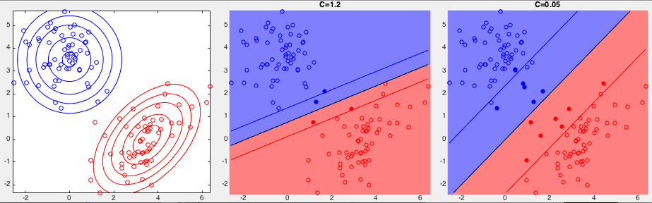
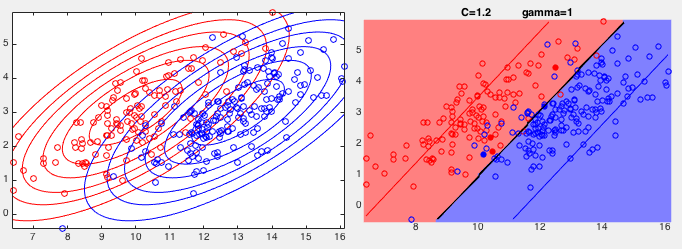
Example 1: The same training set used previously to test the SVM with a hard margin is used again to test the SVM with a soft margin. Two results are shown below, corresponding to two different values $C=1.2$ and $C=0.05$ for the weight of the error term $\sum_{n=1}^N\xi_n$ in the objective function. We see that when $C=1.2$ is large, the number of support vectors (the four solid dots) is small due to the small errors $\xi_n$ allowed, and the decision boundary determined by the these support vectors independent of the rest of the data set (circles) is mostly dictated by the local points close to the boundary, not necessarily a good reflection of the global distribution of the data points. This result is similar to the previous one generated by the hard-margin SVM.

On the other hand, when $C=0.1$ is small, a greater number of data points become support vectors due to the larger (the 13 solid dots) error $\xi_n$ allowed, and the resulting linear decision line determined by these support vectors reflects global distribution of the data points, and it better separates the two classes in terms of their mean positions.

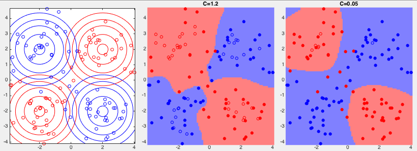
Example 2: The classification results for the XOR data set are shown below with $C=1.2$ and $C=0.05$. As the two classes in the XOR data set are not linearly separable, a Gaussian or radial basis function (RBF) kernel is used to map the data from 2-D space to an infinite dimensional space, which is partitioned into two regions for the two classes. When $C=1.2$ is large, the decision boundary is dictated by a relatively small number of support vectors (solid dots, with small error $\xi_n$) and all data points are classified correctly, but it is more prone to the overfitting problem, if some of the small number of support vectors are outliers due to noise.

One the other hand, when $C=0.05$ is small, the decision boundary is determined by a greater number of support vectors, better reflecting the global distribution of the data points. However, as the local points close to the boundary are not relatively deemphasized, some miss-classification occurs, some nine red dots are classified into the blue region incorrectly.

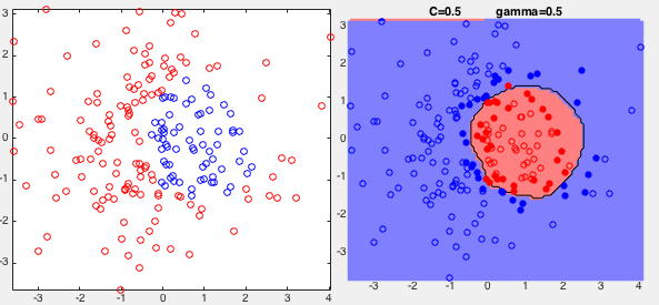
Example 3:

Example 4: