Next: Kernel Mapping Up: Support Vector machine Previous: Support Vector machine
The support vector machine (SVM) is a supervised binary classifier
trained by a dsta set
 of
which data sample
of
which data sample  , a vector in the d-dimensional feature
space, belongs to either class
, a vector in the d-dimensional feature
space, belongs to either class  if labeled by
  or class
 if labeled by
  . The result of the training process is
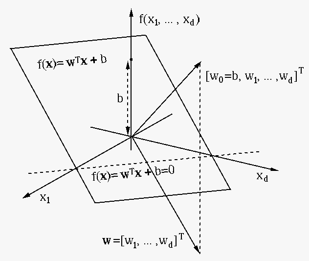
the decision boundaries or decision plane
. The result of the training process is
the decision boundaries or decision plane  in the
feature space, described by the linear decision equation:
in the
feature space, described by the linear decision equation:
 |
(62) |
 and intercept
  . Once
the two parameters and are determined based on the
training set, any unlabeled sample
. Once
the two parameters and are determined based on the
training set, any unlabeled sample  can be classified into
either of the two classes:
can be classified into
either of the two classes:
if then then |
(63) |
The initial setup of the SVM algorithm seems the same as the
method of linear regression
as a linear binary classifier when the linear regression function
 is thresholded by zero to become
 . But here for the SVM, the parameters and
are determined in such a way that the corresponding decision
plane separates the training samples belonging to the two classes
optimally, so that its distance to the closest samples on either
side, called support vectors, is maximized. Also, as kernel
mapping can be applied to the SVM, it can also be used for nonlinear
classification.
. But here for the SVM, the parameters and
are determined in such a way that the corresponding decision
plane separates the training samples belonging to the two classes
optimally, so that its distance to the closest samples on either
side, called support vectors, is maximized. Also, as kernel
mapping can be applied to the SVM, it can also be used for nonlinear
classification.
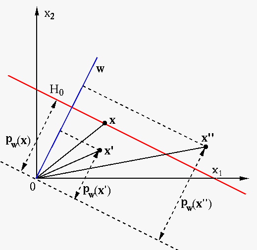
We rewrite the decision equation
 as
as
 |
(64) |
 on the decision plane onto its normal direction ,
of which the absolute value is the distance between and the
origin:
We further find the projection of any point
on the decision plane onto its normal direction ,
of which the absolute value is the distance between and the
origin:
We further find the projection of any point
 off the decision plane onto as
 , and its distance
to as:
, and its distance
to as:
 |
(66) |
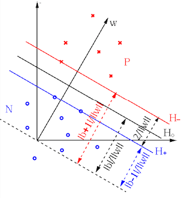
We desire to find the optimal decision plane that separates
the training samples belonging to the two different classes, assumed
to be linearly separable, in such a way that its distance to the
support vectors, denoted by
 , is maximized:
 |
(67) |
 and
and  that
are in parallel with and pass through the support vectors
on either side of :
As these equations can be arbitrarily scaled, we can let
that
are in parallel with and pass through the support vectors
on either side of :
As these equations can be arbitrarily scaled, we can let  for
convenience. Based on Eq. (65), the distances from
or to the origin can be written as
for
convenience. Based on Eq. (65), the distances from
or to the origin can be written as
 |
(69) |
, called the decision
margin, can be found as:
To maximize this margin, we need to minimize
 .
.
For these planes to correctly separate all samples in the training set
 , they have to satisfy the
following two conditions:
, they have to satisfy the
following two conditions:
 |
(71) |
or
, while the inequalities are satisfied by all other samples
farther away from behind or . The two conditions
above can be combined to become:
Now the task of finding the optimal decision plane can be
formulated as a constrained minimization problem:
Example:
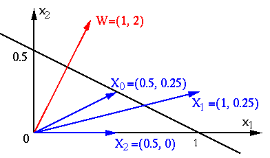
The straight line in 2D space shown above, denoted by ,
is described by the following linear equation
![$\displaystyle f({\bf x})={\bf w}^T{\bf x}+b=[w_1,w_2]
\left[ \begin{array}{c} x...
...b
=[1, 2]\left[ \begin{array}{c} x_1 \\ x_2 \end{array} \right]-1
=x_1+2x_2-1=0$](img290.svg) |
(74) |
to the origin is:
 |
(75) |
![${\bf x}_0=[0.5,\;0.25]^T$](img292.svg) ,
,
 ,
i.e.,
,
i.e.,  is on the plane. Its distance to the plane is
 .
.
![${\bf x}_1=[1,\;0.25]^T$](img296.svg) ,
,
 ,
i.e.,
,
i.e.,  is above the straight line, its distance to the plane
is
is above the straight line, its distance to the plane
is
 .
.
![${\bf x}_2=[0.5,\;0]^T$](img300.svg) ,
,
 , i.e.,
 is below the straight line, its distance to the plane is
 .
.
These two points
![${\bf x}_1=[1,\,0.25]^T$](img304.svg) and
and
![${\bf x}_2=[0.5,\,0]^T$](img305.svg) with equal distance to , the straight line
with equal distance to , the straight line
 ,
can be assumed to be two support vectors
on either side of
, and
,
can be assumed to be two support vectors
on either side of
, and
 |
(76) |
 on both sides of the decision equation
,
it is scaled to become
on both sides of the decision equation
,
it is scaled to become
 |
(77) |
parallel to and passing
through and passing through are
 |
 |
||
 |
 |
 |
(78) |
and is indeed
 :
:
 |
(79) |
and the origin
 found previously.
For reasons to be discussed later, instead of directly solving the constrained minimization problem in Eq. (73), now called the primal problem, we actually solve the dual problem. Specifically, we first construct the Lagrangian function of the primal problem:
where are the Lagrange multipliers,
which is called the primal function. Here for this minimization
problem with non-positive constraints, the Lagrangian multipliers are
required to be negative,
are the Lagrange multipliers,
which is called the primal function. Here for this minimization
problem with non-positive constraints, the Lagrangian multipliers are
required to be negative,  , according to Table
 ![[*]](crossref.png) here, if a minus sign is used
for the second term. However, to be consistent with most SVM literatures,
we use the positive sign for the second term and require
here, if a minus sign is used
for the second term. However, to be consistent with most SVM literatures,
we use the positive sign for the second term and require
 .
Note that if is a support vector on either or ,
i.e., the equality constraint
.
Note that if is a support vector on either or ,
i.e., the equality constraint
 holds, then
 ; but if is not a support vector, the equality
constraint does not hold, and
; but if is not a support vector, the equality
constraint does not hold, and
 .
.
We next find the minimum (or infimum) as the lower bound of the primal
function
 in Eq. (80), by setting to
zero its partial derivatives with respect to both and :
in Eq. (80), by setting to
zero its partial derivatives with respect to both and :
![$\displaystyle \frac{\partial}{\partial {\bf w}}L_p({\bf w},b)
=\frac{\partial}{...
...\bf w}^T {\bf x}_n+b))\right]
={\bf w}-\sum_{n=1}^N\alpha_ny_n{\bf x}_n={\bf0},$](img327.svg) |
(82) |
 , we get its lower bound as a function
of the Lagrange multipliers
, we get its lower bound as a function
of the Lagrange multipliers
 , called
the dual function:
, called
the dual function:
 |
 |
![$\displaystyle \inf_{{\bf w},b} L_p({\bf w},b,{\bf\alpha})
=\inf_{{\bf w},b}\lef...
...}{\bf w}^T{\bf w}
+\sum_{n=1}^N \alpha_n(1-y_n( {\bf w}^T {\bf x}_n+b)) \right]$](img332.svg) |
|
|
![$\displaystyle \inf_{{\bf w},b}\left[\frac{1}{2}{\bf w}^T{\bf w}
+\sum_{n=1}^N \...
...\bf w}^T \sum_{n=1}^N \alpha_ny_n{\bf x}_n
-b\;\sum_{n=1}^N \alpha_ny_n \right]$](img333.svg) |
||
|
 |
||
|
 |
(84) |
 with respect to the Lagrange multipliers, subject to the constraint
imposed by Eq. (81):
with respect to the Lagrange multipliers, subject to the constraint
imposed by Eq. (81):
 is an
is an  by symmetric matrix of which the component
in the mth row and nth column is
by symmetric matrix of which the component
in the mth row and nth column is
 (
(
 ). Now we have converted the primal problem of
constrained minimization of the primal function
with respect to and to its dual problem of linearly
constrained maximization of the dual function
with respect to
. Solving this
quadratic programming (QP) problem,
we get all Lagrange multipliers
). Now we have converted the primal problem of
constrained minimization of the primal function
with respect to and to its dual problem of linearly
constrained maximization of the dual function
with respect to
. Solving this
quadratic programming (QP) problem,
we get all Lagrange multipliers
 .
All training samples corresponding to positive Lagrange
multipliers
are support vectors, while others corresponding
to
are not support vectors.
.
All training samples corresponding to positive Lagrange
multipliers
are support vectors, while others corresponding
to
are not support vectors.
We can now find the normal direction of the optimal decision
plane based on Eq. (83):
is the difference between the
weighted means of the support vectors in class (first term)
and class (second term), and it is determined only by the
support vectors.
Having found
, we can also find
based on the equality of Eq. (72) for any of the
support vectors:
 or or |
(87) |
 ). Solving the equation for we get:
All support vectors should yield the same result. Computationally we
simply get as the average of the above for all support vectors.
). Solving the equation for we get:
All support vectors should yield the same result. Computationally we
simply get as the average of the above for all support vectors.
We note that both and depend only on the support vectors
on planes and , corresponding to a positive
,
while all remaining samples corresponding to
are farther
away from the decision plane , behind either or . We
see that the SVM is solely based on those support vectors in the
training set, once they are identified during the training process,
all other non-support vectors are irrelevant.
Having obtained and as shown above as the training process,
any unlabeled sample can be classified into either of the two
classes depending on whether the following decision function is greater
or smaller than zero:
 |
|
 |
|
|
 |
(90) |
 . Now the decision margin can be written as:
 |
(91) |
The SVM algorithm for binary classification can now by summarized as the following steps:
by solving the QP problem in Eq. (85);
by Eq. (86);
by Eq. (88);
by Eq. (89).
as well as
and  in the training set, the normal vector
is never needed, and the second step above for calculating
by Eq. (86) can be dropped.
in the training set, the normal vector
is never needed, and the second step above for calculating
by Eq. (86) can be dropped.
We prefer to solve this dual problem not only because it is easier
than the original primal problem, but also, more importantly, for
the reason that all data points appear only in the form of an inner
product
 in the dual problem, allowing the
kernel method to be used, as discussed later.
in the dual problem, allowing the
kernel method to be used, as discussed later.
The Matlab code for the essential part of the algorithm is listed
below, where X and y are respectively the data array
composed of training vectors
![$[{\bf x}_1,\cdots,{\bf x}_N]$](img356.svg) and
their corresponding labelings
and
their corresponding labelings
 , and
, and IPmethod
is a function that implements the
interior point method
for solving a general QP problem of minimizing
 subject to the linear
equality constraints
subject to the linear
equality constraints
 and
and
 .
.
    [X y]=getData;               % get the training data
    [m n]=size(X);
    Q=(y'*y).*(X'*X);            % compute the quadratic matrix
    c=-ones(n,1);                % coefficients of linear term
    A=y;                         % coefficient matrix and
    b=0;                         % constants of linear equality constraints
    alpha=0.1*ones(n,1);         % initial guess of solution

    [alpha mu lambda]=IPmethod(Q,A,c,b,alpha);  % solve QP to find alphas
                                                % by interior point method
    I=find(abs(alpha)>10^(-3));  % indecies of non-zero alphas
    asv=alpha(I);                % non-zero alphas
    Xsv=X(:,I);                  % support vectors
    ysv=y(:,I);                  % their labels
    w=sum(repmat(ysv.*asv,m,1).*Xsv,2);  % normal vector (not needed)
    bias=mean(ysv-w'*Xsv);               % bias
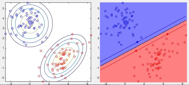
Example: The training set contains two classess of 2-D points with Gaussian distributions generated based on the following mean vectors and covariance matrices:
![$\displaystyle {\bf m}_-=\left[\begin{array}{c}3.5\\ 0\end{array}\right],\;\;\;\...
...y}\right],\;\;\;\;
{\bf S}_+=\left[\begin{array}{cc}1&0\\ 0&1\end{array}\right]$](img361.svg) |
(92) |
and constant
of the optimal boundary between the two classes based on three support
vectors, all listed below. Note that decision boundary is completely
dictated by the three support vectors and the margion distance between
them is maximized.
![\begin{displaymath}\begin{array}{c\vert c\vert l\vert r}\hline
n & \alpha_n & {\...
...rray}{r}-1.25\\ 2.39\end{array}\right],\;\;\;\;\;\;\;\;
b=-1.31\end{displaymath}](img362.svg) |
(93) |


![$\displaystyle \frac{\partial}{\partial b}L_p({\bf w},b)
=\frac{\partial}{\parti...
...}^N \alpha_n(1-y_n( {\bf w}^T {\bf x}_n+b))\right]
=\sum_{n=1}^N \alpha_n y_n=0$](img326.svg)


