Optimization with Equality Constraints

The optimization problems subject to equality constraints can be generally formulated as:

$$\left\{\begin{tabular}{ll} max/min & $f({\bf x})=f(x_1,\cdots,x_N... ...\bf x})=h_i(x_1,\cdots,x_N)=0,\;\;\;\;\;(i=1,\cdots m)$\\ \end{tabular}\right.$$ (173)

where $f({\bf x})$ is the objective function and $h_i({\bf x})=0$ is the ith constraint. Here $m\le N$, as in general there does not exist a solution that satisfies more than $N$ equations in the N-D space.

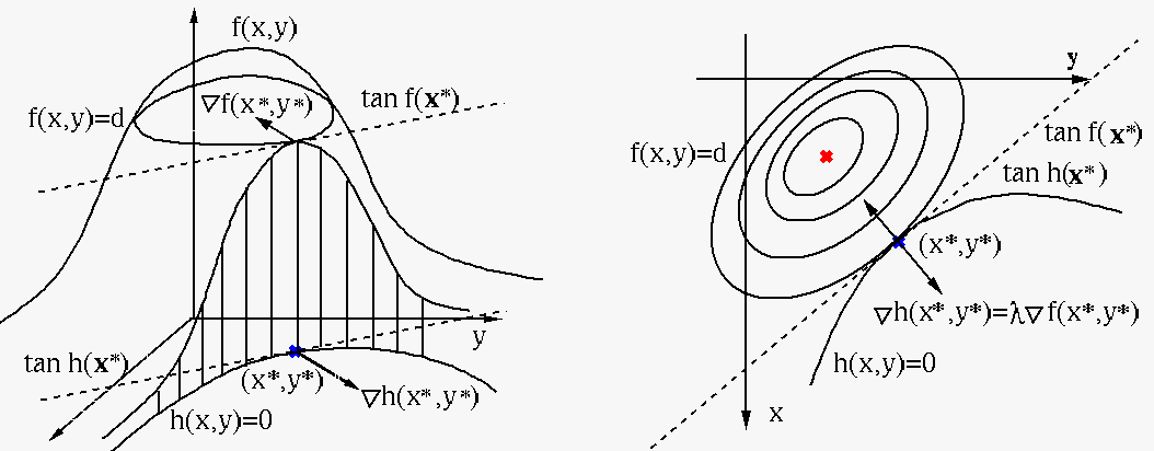
This problem can be visualized in the special case with $N=2$ and $m=1$, where both $f({\bf x})$ and $h({\bf x})$ are surfaces defined over the 2-D space spanned by $x_1$ and $x_2$, and $h({\bf x})=0$ is the intersection line of $h({\bf x})$ and the 2-D plane. The solution ${\bf x}^*$ must satisfy the following two conditions:

• ${\bf x}^*$ is on the intersection line, i.e., $h({\bf x}^*)=0$;
• ${\bf x}^*$ is on the contour line $f({\bf x})=d$ (for some $d$ as shown in the figure), so that $f({\bf x}^*)$ neither increase nor decrease (no point is higher or lower) in the neighborhood of ${\bf x}^*$ along the contour line.

For both conditions to be satisfied, the two contours $h({\bf x})=0$ and $f({\bf x})=d$ must coincide at ${\bf x}^*$, i.e., they must have the same tangents and therefore parallel gradients (perpendicular to the tangents):

$$\bigtriangledown_{\bf x}f({\bf x}^*) =\lambda\,\bigtriangledown_{\bf x} h({\bf x}^*)$$ (174)

where $\bigtriangledown_{\bf x}f({\bf x})=[\partial f/\partial x_1, \cdots,\partial f/\partial x_N ]^T$ is the gradient of $f({\bf x})$, and $\lambda$ is a constant scaling factor which can be either positive if the two gradients are in the same direction or negative if they are in opposite directions. As here we are only interested in whether the two curves coincide or not, the sign of $\lambda^*$ can be either positive or negative.

To find such a point ${\bf x}^*$, we first construct a new objective function, called the Lagrange function (or simply Lagrangian):

$$L({\bf x},\lambda)=f({\bf x})-\lambda\, h({\bf x})$$ (175)

where $\lambda$ is the Lagrange multiplier, which can be either positive or negative (i.e., the sign in front of $\lambda$ can be either plus or minus), and then set the gradient of this objective function with respect to $\lambda$ as well as ${\bf x}$ to zero:

$$\bigtriangledown_{{\bf x},\lambda} L({\bf x},\lambda) =\bigtriangledown_{{\bf x},\lambda} [ f({\bf x})-\lambda\, h({\bf x}) ] ={\bf0}$$ (176)

This equation contains two parts:

$$\left\{\begin{array}{l} \bigtriangledown_{\bf x} f({\bf x})=\lamb... ...=\partial L({\bf x},\lambda)/\partial \lambda =-h({\bf x})=0 \end{array}\right.$$ (177)

This is an equation system containing $N+m=2+1=3$ equations for the same number of unknowns $x_1,\,x_2,\,\lambda$:

$$\frac{\partial f({\bf x})}{\partial x_i} =\lambda \frac{\partial h({\bf x})}{\partial x_i}\;\;\;(i=1,2), \;\;\;\;\;h({\bf x})=0$$ (178)

The solution ${\bf x}^*=[x_1^*,\,x_2^*]^T$ and $\lambda^*$ of this equation system happens to satisfy the two desired relationships: (a) $\bigtriangledown_{\bf x}f({\bf x})=\lambda\bigtriangledown_{\bf x}h({\bf x})$, and (b) $h({\bf x}^*)=0$.

Specially, consider the following two possible cases:

• If $\lambda^*=0$, then $\bigtriangledown_{\bf x}f({\bf x}^*)=\lambda^*\bigtriangledown_{\bf x}h({\bf x}^*)=0$, indicating $f({\bf x}^*)$ is an extremum independent of the constraint, i.e., the constraint $h({\bf x})=0$ is inactive, and the optimization is unconstrained.
• If $\lambda^*\ne 0$, then $\bigtriangledown_{\bf x}f({\bf x}^*)\ne 0$ (as in general $\bigtriangledown_{\bf x}h({\bf x}^*)\ne{\bf0}$), indicating $f({\bf x}^*)$ is not an extremum without the constraint, i.e., the constraint is active, and the optimization is indeed constrained.

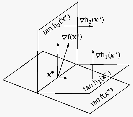
The discussion above can be generalized from 2-D to an $N>2$ dimensional space, in which the optimal solution ${\bf x}^*$ is to be found to extremize the objective $f({\bf x})$ subject to $m$ equality constraints $h_i({\bf x})=0\;(i=1,\cdots,m)$, each representing a contour surface in the N-D space. The solution ${\bf x}^*$ must satisfy the following two conditions:

• ${\bf x}^*$ is on all $m$ contour surfaces so that $h_1({\bf x}^*)=\cdots=h_m({\bf x}^*)=0$, i.e., it is on the intersection of these surfaces, a curve in the space (e.g., the intersection of two surfaces in 3-D space is a curve);
• ${\bf x}^*$ is on a contour surface $f({\bf x}^*)=d$ (for some value $d$) so that $f({\bf x}^*)$ is an extremum, i.e., it does not increase or degrease in the neighborhood of ${\bf x}^*$ along the curve.

Combining these conditions, we see that the intersection (a curve or a surface) of the $m$ surfaces $h_i({\bf x})=0$ must coincide with the contour surface $f({\bf x})=d$ at ${\bf x}^*$, i.e., the intersection of the tangent surfaces of $h_i({\bf x})=0$ through ${\bf x}^*$ must coincide with the tangent surface of $f({\bf x})=d$ at ${\bf x}^*$, therefore the gradient $\bigtriangledown f({\bf x}^*)$ must be a linear combination of the $m$ gradients $\bigtriangledown h_i({\bf x}^*)$:

$$\bigtriangledown_{\bf x}f({\bf x}^*) =\sum_{i=1}^m \lambda_i^* \bigtriangledown_{\bf x} h_i({\bf x}^*)$$ (179)

To find such a solution ${\bf x}^*$ of the optimization problem, we first construct the Lagrange function:

$$L({\bf x},{\bf\lambda})=f({\bf x})-\sum_{i=1}^m\lambda_i h_i({\bf x})$$ (180)

where ${\bf\lambda}=[\lambda_1,\cdots,\lambda_m]^T$ is a vector for $m$ Lagrange multipliers, and then set its gradient to zero:

$$\bigtriangledown_{{\bf x},{\bf\lambda}} L({\bf x},{\bf\lambda}) =... ...\lambda}} \left[ f({\bf x})-\sum_{i=1}^m \lambda_i h_i({\bf x}) \right] ={\bf0}$$ (181)

to get the following two equation systems of $N$ and $m$ equations repectively:

$$\bigtriangledown_{\bf x} f({\bf x}) =\sum_{i=1}^m \lambda_i \bigtriangledown_{\bf x} h_i({\bf x}) \;\;\;\; \;\;\;\; \frac{\partial f({\bf x})}{\partial x_j} =\sum_{i=1}^m\lambda_i \frac{\partial h_i({\bf x})}{\partial x_j} \;\;\;(j=1,\cdots,N),$$ (182)

and

$$\frac{\partial L({\bf x},{\bf\lambda})}{\partial \lambda_i} =h_i({\bf x})=0\;\;\;\;(i=1,\cdots,m)$$ (183)

The first set of $N$ equations indicates that the gradient $\bigtriangledown_{\bf x}f({\bf x}^*)$ at ${\bf x}^*$ is a linear combination of the $m$ gradients $\bigtriangledown_{\bf x} h_i({\bf x}^*)$, while the second set of $m$ equations guarantees that ${\bf x}^*$ also satisfy the $m$ equality constraints. Solving these equations we get the desired soluton ${\bf x}^*$ together with the Lagrange multipliers $\lambda_1,\cdots,\lambda_m$. This is the Lagrange multiplier method.

Specially, if $\lambda_i=0$, then the ith constraint is not active. More specially if $\lambda_i=0$ for all $i=1,\cdots,m$, then

$$\bigtriangledown_{\bf x} f({\bf x}^*) =\sum_{i=1}^m \lambda_i \bigtriangledown_{\bf x} h_i({\bf x})={\bf0}$$ (184)

indicating $f({\bf x}^*)$ is an extremum independent of any of the constraints, i.e., ${\bf x}^*$ is an unconstrained solution, and the optimization problem is unconstrained.