Policy Gradient Methods

All RL algorithms previous considered are based on either state or action-value function and the policy is indectly derived from them by greedy or $\epsilon$-greedy method. However, as the ultimate goal of an RL problem is to find the optimal policy that maximizes the return, it make sense to consider this as an optimization problem to directly find the optimal policy based on an objective function representing the total return to be maximized, by the gradient ascent method, as discussed in the following.

Previously we approximate the state value function $v_\pi(s)$ and action value function $q_\pi(s,a)$ by some parameterized functions $\hat{v}_\pi(s,{\bf w})$ and $\hat{q}_\pi(s,a,{\bf w})$ respectively, of which the parameter ${\bf w}$ can be obtained by sampling the environment, as a supervised learning process. Now we construct a model of a stochastic policy as a parameterized function:

$$\pi(a\vert s,{\bf\theta})=P(a\vert s,{\bf\theta})$$ (110)

where vector ${\bf\theta}=[\theta_1,\cdots,\theta_d]^T$ represents some $d$ parameters of the model. As the dimensionality $d$ is typically smaller than the number of states and actions, such a parameterized policy model is suitable in cases where the numbers of states and actions are large or even continuous.

As a specific example, the policy model can be based on the soft-max function:

$$\pi(a\vert s,{\bf\theta})=\frac{e^{h(s,a,\theta)}}{\sum_be^{h(s,b,\theta)}}$$ (111)

satisfying $\sum_a\pi(a\vert s,{\bf\theta})=1$. Here the summation is over all possible actions, and $h(s,a,\theta)$ is the preference of action $a$ in state $s$, which can be a parameterized function such as a simple linear function $h(s,a,\theta)={\bf\theta}^T{\bf x}(s,a)$, or a neural network with weights represented by ${\bf\theta}$, the same as how the value functions are approxmiated in Section 1.5. According to this policy, an action with higher preference $h(s,a,\theta)$ will have a higher probability to be chosen.

Different from how we find the parameter ${\bf w}$ of $\hat{q}(s,a,{\bf w})$ by minimizing $J({\bf w})$, the mean squared error between the value function $q_\pi(s,a)$ and its model $\hat{q}_\pi(s,a,{\bf w})$, based on gradient descent, here we find the parameter ${\bf\theta}$ of $\pi(a\vert s,{\bf\theta})$ by maximizing $J({\bf\theta})$ representing the value function, the expected return, under the policy, based on gradient ascent. Such methods are therefore called policy gradient methods.

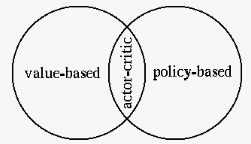
The value-function based methods considered previously and the policy-based methods considered here are summarized below, together with the actor-critic method, as the combination of the two:

• Value-based: the policy is derived by the greedy or $\epsilon$-greedy method based on the value function learned during sampling the environment as a supervised learning process.

• Policy-based: the policy is directly learned without explicitly value functioin estimation.

• Actor-Critic: parameters for both the value function model and policy model are learned simultaneously.

Advantages of policy-based RL includes better convergence properties, but may stuck at local optimum, effective in high-dimensional or continuous action space can learn stochastic policies, but have high variance.

How good a policy is may be measured by different objective functions all related to the values or rewards associated with the policy being evaluated, depending on the environment of the specific problem:

• In episodic environments with finite horizon, we can use the value, the expected return (sum of discounted future rewards), of the start state $s_0$:

  $$J_1(\theta)=v_{\pi_\theta}(s_0)$$ (112)

• In continuing (online) environments with infinite horizon, we can use the average value

  $$J_{avV}(\theta)=\sum_s d_{\pi_\theta}(s) v_{\pi_\theta}(s)$$ (113)

  where $d_{\pi_\theta}(s)$ is the stationary distribution of all states under policy $\pi(a\vert s,\theta)$.

We can find the optimal paramter ${\bf\theta}^*$ for the policy model $\pi(a\vert s,{\bf\theta})$ by solving the maximization problem:

$$\theta^*=\argmax_\theta J(\theta)$$ (114)

based on the gradient of $J(\theta)$:

$$\triangledown_\theta J(\theta)=\frac{d}{d{\theta}}J(\theta) =\lef... ...rtial J}{\partial\theta_1},\cdots, \frac{\partial J}{\partial\theta_n}\right]^T$$ (115)

by the iterative gradient ascent method:

$${\bf\theta}_{t+1}={\bf\theta}_t+\Delta{\bf\theta} ={\bf\theta}_t+\alpha \triangledown_\theta J({\bf\theta})$$ (116)

Here we use $t$ for the index of the iteration based on the assumption that the a new sample point is available at every time step of an episode while sampling the environment following policy $\pi(a\vert s,{\bf\theta})$.

While it is conceptually straight forward to see how gradient ascent method can be used to find the optimal parameter ${\bf\theta}^*$ that maximizes $J({\bf\theta})$, it is not easy to actually find its gradient $\triangledown J({\bf\theta})$, which depends on not only what actions to take at the states directly determined by the policy $\pi(a\vert s,{\bf\theta})$, but also how the states are distributed under the policy in an unknown environment. This challenge is addressed by the following policy gradient theorem. The proof of the theorem below leads to an expression of the gradient $\triangledown_\theta J({\bf\theta})$, which can be used to find the optimal parameter ${\bf\theta}^*$ iteratively by the stochastic gradient ascend method.

Proof of policy gradient theorem:

$$\triangledown_\theta v_{\pi_\theta}(s) = \triangledown_\theta \left(\sum_a \pi(a\vert s,{\bf\theta})q_{\pi_\theta}(s,a)\right)$$

$$\stackrel{1}{=} \sum_a \left[ \triangledown_\theta\pi(a\vert s,{\bf\theta})\;q_{\... ...,a) +\pi(a\vert s,{\bf\theta})\;\triangledown_\theta q_{\pi_\theta}(s,a)\right]$$

$$\stackrel{2}{=} \sum_a \left[ \triangledown_\theta\pi(a\vert s,{\bf\theta})\;q_{\... ...iangledown_\theta\sum_{s'}\sum_r P(s',r\vert s,a)(r+v_{\pi_\theta}(s')) \right]$$

$$\stackrel{3}{=} \sum_a \left[ \triangledown_\theta\pi(a\vert s,{\bf\theta})\;q_{\... ...\sum_{s'}\sum_rP(s',r\vert s,a) \triangledown_\theta v_{\pi_\theta}(s') \right]$$

$$\stackrel{4}{=} \sum_a \left[ \triangledown_\theta\pi(a\vert s,{\bf\theta})\;q_{\... ...f\theta})\sum_{s'}P(s'\vert s,a)\triangledown_\theta v_{\pi_\theta}(s') \right]$$

$$\stackrel{5}{=} \sum_a \triangledown_\theta\pi(a\vert s,{\bf\theta})\;q_{\pi_\the... ...}\pi(a\vert s,{\bf\theta})P(s'\vert s,a)\triangledown_\theta v_{\pi_\theta}(s')$$

$$\stackrel{6}{=} \phi(s)+\sum_{s'}\sum_a P(s'\vert s,a)\pi(a\vert s,{\bf\theta})\triangledown_\theta v_{\pi_\theta}(s')$$ (117)

where

1. product rule of derivative: $(uv)'=u'v+uv'$
2. $q_{\pi_\theta}(s,a)=\sum_{s'}\sum_rP(s',r\vert s,a)(r+v_{\pi_\theta}(s'))$
3. $r$ is not a function of $\theta$
4. $\sum_rP(s',r\vert s,a)=P(s'\vert s,a)$ in Eq. (17)
5. $\pi(a\vert s,{\bf\theta})$ is indpendent of $s'$ and moved inside summation over $s'$
6. We have defined

   $$\phi(s)=\sum_a\triangledown_\theta\pi(a\vert s,{\bf\theta})\;q_{\pi_\theta}(s,a)$$ (118)

We note that Eq. (refPolicyGradientThm1) is a recursion by which $\triangledown_\theta v_{\pi_\theta}(s)$ is expressed as a function in terms $\triangledown_\theta v_{\pi_\theta}(s')$.

We further define $Pr_\pi(s\rightarrow x,k)$ as the probability of transitioning from state $s$ to a state $x$ after $k$ steps following $\pi(a\vert s,\theta)$:

$$s\stackrel{\pi(a\vert s,{\bf\theta})}{\longrightarrow}s' \stackre... ...} \cdots \stackrel{\pi(a\vert s^{(k-1)},{\bf\theta})}{\longrightarrow}s^{(k)}=x$$ (119)

with the following properties:

• $$Pr_\pi(s\rightarrow s,0)=1$$ (120)

• $$Pr_\pi(s\rightarrow s',1)=\sum_a\pi(a\vert s,{\bf\theta})P(s'\vert s,a)$$ (121)

• $$\sum_{s'}Pr_\pi(s\rightarrow s',1)=1$$ (122)

• $$Pr_\pi(s\rightarrow s'',2) =Pr_\pi(s\rightarrow s',1) Pr_\pi(s'\rightarrow s'',1)$$ (123)

Continuing Eq. (117) we keep rolling out the recursion of $\triangledown_\theta v_{\pi_\theta}(s')$ and get:

$$\triangledown_\theta v_{\pi_\theta}(s) = \phi(s)+\sum_{s'}\sum_a\pi(a\vert s,{\bf\theta}) P(s'\vert s,a)\triangledown_\theta v_{\pi_\theta}(s')$$

$$\stackrel{1}{=} \phi(s)+\sum_{s'}Pr_\pi(s\rightarrow s',1)\triangledown_\theta v_{\pi_\theta}(s')$$

$$\stackrel{2}{=} \phi(s)+\sum_{s'}Pr_\pi(s\rightarrow s',1) \left[ \phi(s')+\sum_{s''}Pr_\pi(s'\rightarrow s'',1)\triangledown_\theta v_{\pi_\theta}(s'')\right]$$

$$\stackrel{3}{=} \phi(s)+\sum_{s'}Pr_\pi(s\rightarrow s',1)\phi(s') +\sum_{s''}Pr_... ...arrow s',1) Pr_\pi(s'\rightarrow s'',1)\triangledown_\theta v_{\pi_\theta}(s'')$$

$$\stackrel{4}{=} \phi(s)+\sum_{s'}Pr_\pi(s\rightarrow s',1)\phi(s') +\sum_{s''}Pr_\pi(s\rightarrow s'',2) \triangledown_\theta v_{\pi_\theta}(s'')$$

$$\stackrel{5}{=} \phi(s)+\sum_{s'}Pr_\pi(s\rightarrow s',1)\phi(s') +\sum_{s''}Pr_... ...sum_{s'''}Pr_\pi(s\rightarrow s''',2) \triangledown_\theta v_{\pi_\theta}(s''')$$

$$= \cdots\cdots \stackrel{6}{=}\sum_{x\in S}\sum_{k=0}^\infty Pr_\pi(s\rightarrow x,k)\phi(x)$$ (124)

where

1. Eq. (121)
2. unroll $\triangledown_\theta v_{\pi_\theta}(s')$
3. Eq. (122)
4. Eq. (123)
5. unroll $\triangledown_\theta v_{\pi_\theta}(s'')$
6. keep unrolling recursively to infinity, and Eq. (120)

Now the gradient of the objective $J(\theta)=v_{\pi_\theta}(s_0)$ can be written as

$$\triangledown_\theta J(\theta) = \triangledown_\theta v_\pi(s_0) =\sum_{s\in S}\sum_{k=0}^\infty Pr_\pi(s_0\rightarrow s,k)\;\phi(s)$$

$$= \sum_{s\in S}\eta(s)\;\phi(s) =\left(\sum_{s'}\eta(s')\right) \sum_{s\in S}\frac{\eta(s)}{\sum_{s'}\eta(s')}\;\phi(s)$$

$$\propto \sum_{s\in S}\frac{\eta(s)}{\sum_{s'}\eta(s')}\;\phi(s) =\sum_{s\... ...(s) \; \sum_a\triangledown_\theta\pi(a\vert s,{\bf\theta})\;q_{\pi_\theta}(s,a)$$ (125)

Here the proportionality is introduced due to the dropping of $\sum_{s'}\eta(s')$ as a constant independent of state $s$, and we also defined

$$\eta(s)=\sum_{k=0}^\infty Pr_\pi(s_0\rightarrow s,k),$$ (126)

as the sum of all probabilities for visiting state $s$ from the start state $s_0$, and

$$\mu_\pi(s)=\frac{\eta(s)}{\sum_{s'}\eta(s')}$$ (127)

as a normalized verion of $\eta(s)$ representing the probability distribution of visiting state $s$ while following policy $\pi$. Eq. (125) can be further written as

$$\triangledown_\theta J(\theta)=\triangledown_\theta v_\pi(s_0) \propto \sum_{s\in S} \mu_\pi(s) \; \sum_a \pi(a\vert s,{\bf\theta}) \fra... ...heta\pi(a\vert s,{\bf\theta})}{\pi(a\vert s,{\bf\theta})}\; q_{\pi_\theta}(s,a)$$

$$= \sum_{s\in S} \mu_\pi(s) \;\sum_a \pi(a\vert s,{\bf\theta})\; \triangledown_\theta\ln \pi(a\vert s,{\bf\theta})\,q_{\pi_\theta}(s,a)$$

$$= E_{\pi_\theta} \left[\triangledown_\theta \ln \pi(a\vert s,{\bf\theta})\,q_{\pi_\theta}(s,a) \right]$$ (128)

where $E_{\pi_\theta}$ denotes the expectation over all actions in each state $s$ weighted by $\pi(a\vert s,{\bf\theta})$ and all states $s\in S$ weighted by $\mu_\pi(s)$.

Q.E.D.

We see that the gradient $\triangledown_\theta J(\theta)$ is now expressed as the expectation of the action value function $q_\pi(s,a)$, weighted by the gradient of the logrithm of the corresponding policy $\pi(a\vert s,{\bf\theta})$. Now Eq. (116) can be further written as

$${\bf\theta}_{t+1} ={\bf\theta}_t+\alpha\triangledown_\theta J({\b... ...\theta}(s_t,a_t)\;\triangledown_\theta \ln \pi(a_t\vert s_t,{\bf\theta})\right]$$ (129)

We further note that Eq. (125) still hold if an arbitrary bias term $b(s)$ independent of action $a$ is included:

$$\triangledown_\theta J(\theta) \propto \sum_{s\in S} \mu_\pi(s) \; \sum_a\triangledown_\theta\pi(a\vert s,{\bf\theta})\;(q_{\pi_\theta}(s,a))$$

$$= \sum_{s\in S} \mu_\pi(s) \; \sum_a\triangledown_\theta\pi(a\vert s,{\bf\theta})\;(q_{\pi_\theta}(s,a)+b(s))$$ (130)

as

$$\sum_a\triangledown_\theta\pi(a\vert s,{\bf\theta})\;b(s) =b(s) \triangledown_\theta\sum_a\pi(a\vert s,{\bf\theta}) =b(s) \triangledown_\theta 1=0$$ (131)

Now Eq. (116) can also be written as

$${\bf\theta}_{t+1} ={\bf\theta}_t+\alpha\triangledown_\theta J({\b... ...s_t,a_t)+b(s_t))\;\triangledown_\theta \ln \pi(a_t\vert s_t,{\bf\theta})\right]$$ (132)

The expectation $E_{\pi_\theta}$ in Eqs. (129) and (132) can be dropped if the method of stochastic gradient ascent is used, as in all algorithms below, where each iterative step is based on only one sample data point instead of its expectation.

Specifically, for a soft-max policy model as given in Eq. (111), we have

$$\triangledown_\theta \ln\pi(a\vert s,{\bf\theta}) = \triangledown_\theta\ln\left( \frac{e^{\theta^T{\bf x}(s,a) }}{\s... ...wn_\theta\left( \theta^T{\bf x}(s,a) -\ln\sum_b e^{\theta^T{\bf x}(s,b)}\right)$$

$$= {\bf x}(s,a)-\frac{\triangledown_\theta \sum_be^{\theta^T{\bf x}(... ...{\sum_b e^{\theta^T{\bf x}(s,b)} {\bf x}(s,b)}{\sum_b e^{\theta^T{\bf x}(s,b)}}$$

$$= {\bf x}(s,a)-\sum_b \frac{e^{\theta^T{\bf x}(s,b)}}{\sum_b e^{\theta^T{\bf x}(s,b)}} {\bf x}(s,b)$$

$$= {\bf x}(s,a)-\sum_b\pi(b\vert s,{\bf\theta}){\bf x}(s,b)$$ (133)

We list set of popular policy-based algorithms below, based on either the MC or TD methods, generally used in previous algorithms.

• REINFORCE (MC) policy gradient

  In this algorithm, the action value function $q_{\pi_\theta}(s_t,a_t)$ in Eq. (129) is replaced by the return $G_t$ btained at the end of each episode while sampling the environment. Now the equation becomes:

  $$\theta_{t+1}=\theta_t+\alpha\gamma^t G_t\;\triangledown_\theta\ln \pi(a\vert s,{\bf\theta})$$ (134)

  Note that the discount factor $\gamma^t$ is included as the expression for $\triangledown_\theta J(\theta)$ in Eq. (128) assumed $\gamma=1$ for simplicity.

  Here is the pseudo code for the algorithm:

  Initialize $\pi(a\vert s,{\theta}$

  loop (for each episode)

  At the end of episode, get $G_t$ for each state visited

  for $t=1,\cdots,T$

  $\theta=\theta+\alpha\gamma^t G_t\triangledown_\theta\ln\pi(a_t\vert s_t,{\bf\theta})$

  end loop

• Actor-Critic (TD) policy gradient

  As its name suggests, this algorithm is based on two approximation function models, the first for the policy $\pi(a\vert s,{\bf\theta})$ parameterized by ${\bf\theta}$, the actor, same as in the REINFORCE algorithm above, and the second for the value function $\hat{v}_\pi(s,{\bf w})$ parameterized by ${\bf w}$, the critic, same as in Eq. (97).

  Specifically, in Eq. (132), the action value function $q_{\pi_\theta}(s_t,a_t)$ is replaced by its bootstrapping expression $r_{t+1}+\gamma \hat{v}_\pi(s',{\bf w})$, and the bias term $b(s)$ is replaced by the approximated value function $\hat{v}(s_t,{\bf w})$. Now both parameters ${\bf w}$ and ${\bf\theta}$ can be found iteratively at every step of an episode while sampling the environment (the TD method) by stochastic gradient method with the expectation $E_\pi$ dropped:
  

  $${\bf w}_{t+1} = {\bf w}_t+\alpha_w \left[ (r_{t+1}+\gamma\hat{v}_\pi(s',{\bf w})-\hat{v}_\pi(s,{\bf w})) \,\triangledown_w\hat{v}_\pi(s,{\bf w})\right]$$

  $$\theta_{t+1} = \theta_t+\alpha_\theta \left[ (r_{t+1}+\gamma\hat{v}_\pi(s',{\bf ... ...t{v}_\pi(s,{\bf w})) \,\triangledown_\theta\ln \pi(a\vert s,{\bf\theta})\right]$$ (135)

  
  

  Here is the pseudo code for the algorithm:

  initialize model parameters ${\bf\theta}$ and ${\bf w}$

  initialize step sizes $\alpha_\theta$ and $\alpha_w$

  loop (for each episode)

  initialize $s=s_0$, $t=0$

  while $s$ is not terminal (for each step)

  take action $a$ following $\pi(a\vert s,{\bf\theta})$, find reward $r$ and next state $s'$

  find TD error: $\delta=r+\gamma\hat{v}(s',{\bf w})-\hat{v}(s,{\bf w})$

  ${\bf w}={\bf w}+\alpha_w\;\delta\;\triangledown\hat{v}(s,{\bf w})$

  ${\bf\theta}={\bf\theta}+\alpha_\theta\gamma^t\delta\;\triangledown\ln \pi(a\vert s,{\bf\theta})$

  $s=s'$

  $t=t+1$

  end while

  end loop

• Backward view of TD($\lambda$) policy gradient

  Here is the pseudo code for the algorithm:

  initialize model parameters ${\bf\theta}$ and ${\bf w}$

  initialize step sizes $\alpha_\theta$ and $\alpha_w$

  initialize trace-decay rates $\lambda_\theta$ and $\lambda_w$

  loop (for each episode)

  initialize $s=s_0$, $t=0$

  initialize ${\bf z}_\theta={\bf0}$, ${\bf z}_w={\bf0}$

  while $s$ is not terminal (for each step)

  take action $a$ following $\pi(a\vert s,{\bf\theta})$, find reward $r$ and next state $s'$

  find TD error: $\delta=r+\gamma\hat{v}(s',{\bf w})-\hat{v}(s,{\bf w})$

  ${\bf z}_\theta=\gamma\lambda_\theta{\bf z}_\theta +\triangledown \gamma^t \ln\pi(a\vert s,{\bf\theta})$

  ${\bf z}_w=\gamma\lambda_w{\bf z}_w +\gamma^t\triangledown\hat{v}(s,{\bf w})$

  ${\bf w}={\bf w}+\alpha_w\;\delta\;\triangledown\hat{v}(s,{\bf w})$

  ${\bf\theta}={\bf\theta}+\alpha_\theta\,\delta\;\triangledown\ln \pi(a\vert s,{\bf\theta})$

  $s=s'$

  $t=t+1$

  end while

  end loop

Following the similar steps, the policy gradient theorem for environment with continuous state and action spaces can be also proven:

$$\triangledown_\theta J(\theta) =\int_s \mu_\pi(s) \;\int_a\triangledown_\theta\pi(a\vert s,{\bf\theta})\;q_{\pi_\theta}(s,a) da\;ds$$ (136)